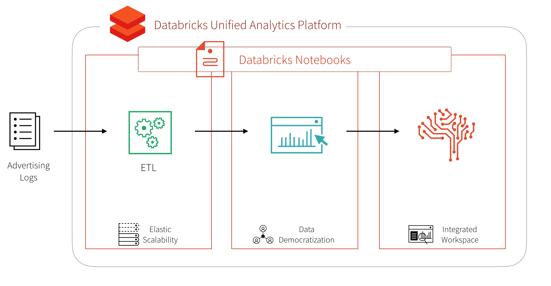
Advertising teams want to analyze their immense stores and varieties of data requiring a scalable, extensible, and elastic platform. Advanced analytics, including but not limited to classification, clustering, recognition, prediction, and recommendations allow these organizations to gain deeper insights from their data and drive business outcomes. As data of various types grow in volume, Apache Spark provides an API and distributed compute engine to process data easily and in parallel, thereby decreasing time to value. The Databricks Unified Analytics Platform provides an optimized, managed cloud service around Spark, and allows for self-service provisioning of computing resources and a collaborative workspace.
Let’s look at a concrete example with the Click-Through Rate Prediction dataset of ad impressions and clicks from the data science website Kaggle. The goal of this workflow is to create a machine learning model that, given a new ad impression, predicts whether or not there will be a click.
To build our advanced analytics workflow, let’s focus on the three main steps:
- ETL
- Data Exploration, for example, using SQL
- Advanced Analytics / Machine Learning
Building the ETL process for the advertising logs
First, we download the dataset to our blob storage, either AWS S3 or Microsoft Azure Blob storage. Once we have the data in blob storage, we can read it into Spark.
%scala
// Read CSV files of our adtech dataset
val df = spark.read
  .option("header", true)
  .option("inferSchema", true)
  .csv("/mnt/adtech/impression/csv/train.csv/")
This creates a Spark DataFrame – an immutable, tabular, distributed data structure on our Spark cluster. The inferred schema can be seen using .printSchema().
%scala
df.printSchema()

# Output
id: decimal(20,0)
click: integer
hour: integer
C1: integer
banner_pos: integer
site_id: string
site_domain: string
site_category: string
app_id: string
app_domain: string
app_category: string
device_id: string
device_ip: string
device_model: string
device_type: integer
device_conn_type: integer
C14: integer
C15: integer
C16: integer
C17: integer
C18: integer
C19: integer
C20: integer
C21: integer
To optimize the query performance from DBFS, we can convert the CSV files into Parquet format. Parquet is a columnar file format that allows for efficient querying of big data with Spark SQL or most MPP query engines. For more information on how Spark is optimized for Parquet, refer to How Apache Spark performs a fast count using the Parquet metadata.
%scala
// Create Parquet files from our Spark DataFrame
df.coalesce(4)
  .write
  .mode("overwrite")
  .parquet("/mnt/adtech/impression/parquet/train.csv")
Explore Advertising Logs with Spark SQL
Now we can create a Spark SQL temporary view called impression on our Parquet files. To showcase the flexibility of Databricks notebooks, we can specify to use Python (instead of Scala) in another cell within our notebook.
%python
# Create Spark DataFrame reading the recently created Parquet files
impression = spark.read \\
.parquet("/mnt/adtech/impression/parquet/train.csv/")

# Create temporary view
impression.createOrReplaceTempView("impression")
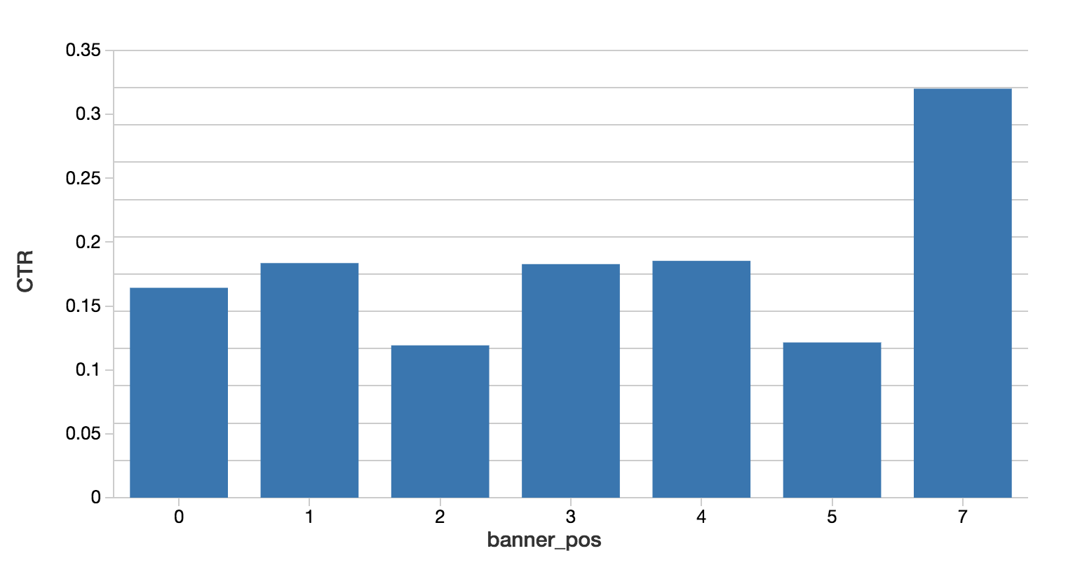
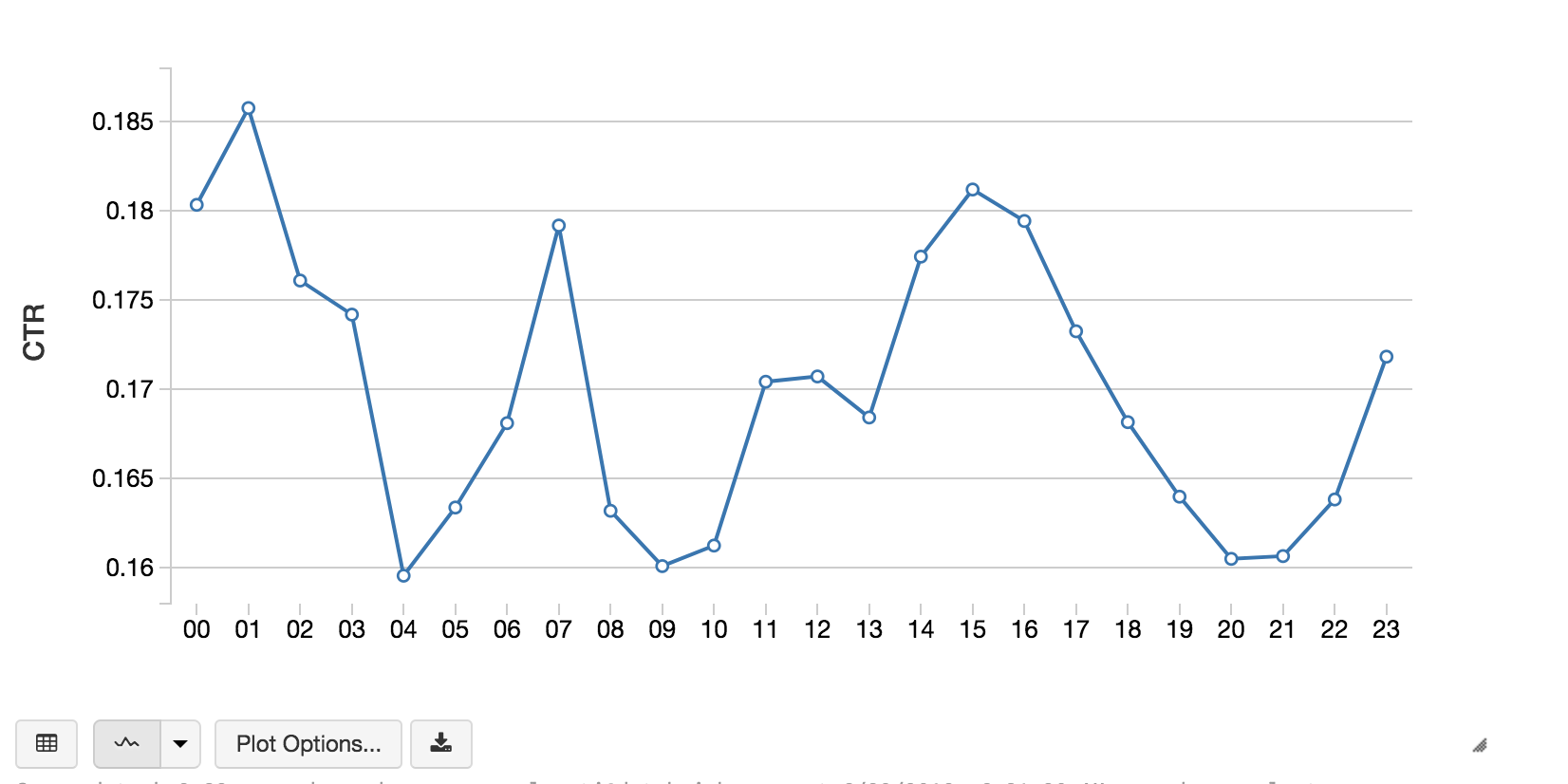
We can now explore our data with the familiar and ubiquitous SQL language. Databricks and Spark support Scala, Python, R, and SQL. The following code snippets calculates the click through rate (CTR) by banner position and hour of day.
%sql
-- Calculate CTR by Banner Position
select banner_pos,
sum(case when click = 1 then 1 else 0 end) / (count(1) * 1.0) as CTR
from impression
group by 1
order by 1
%sql
-- Calculate CTR by Hour of the day
select substr(hour, 7) as hour,
sum(case when click = 1 then 1 else 0 end) / (count(1) * 1.0) as CTR
from impression
group by 1
order by 1
Predict the Clicks
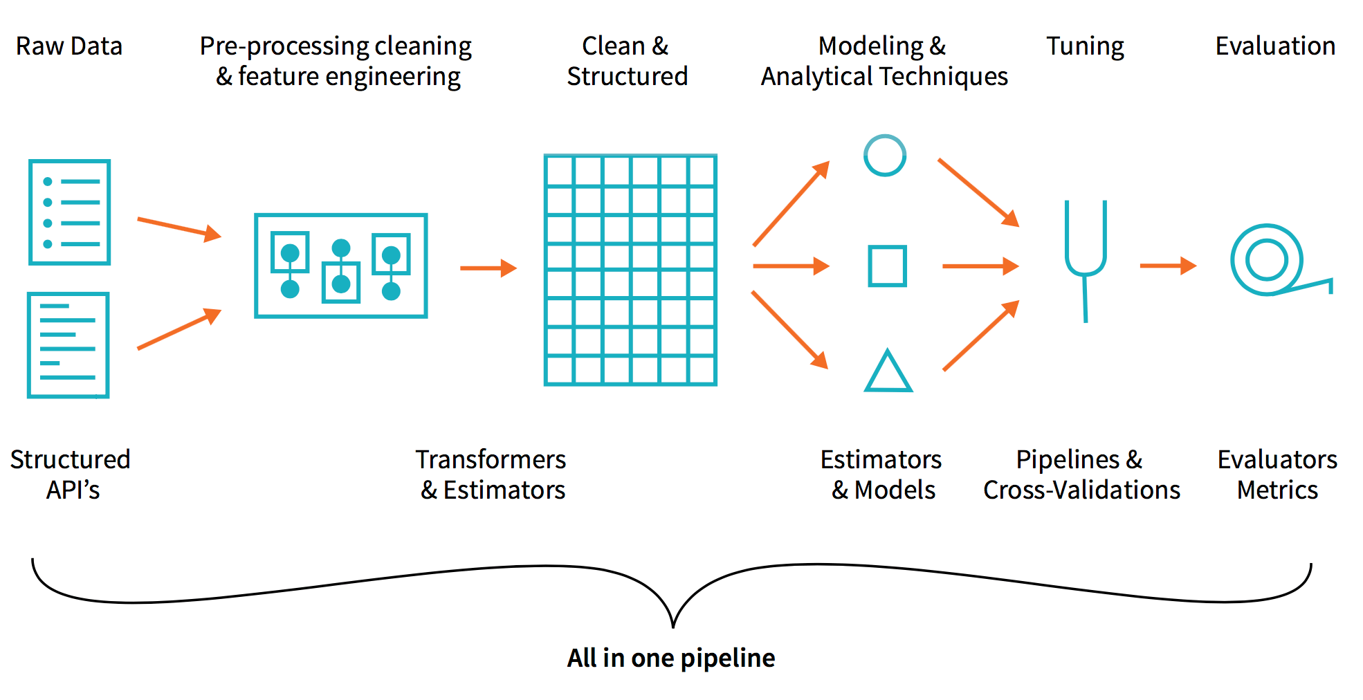
Once we have familiarized ourselves with our data, we can proceed to the machine learning phase, where we convert our data into features for input to a machine learning algorithm and produce a trained model with which we can predict. Because Spark MLlib algorithms take a column of feature vectors of doubles as input, a typical feature engineering workflow includes:
- Identifying numeric and categorical features
- String indexing
- Assembling them all into a sparse vector
The following code snippet is an example of a feature engineering workflow.
# Include PySpark Feature Engineering methods
from pyspark.ml.feature import StringIndexer, VectorAssembler


# All of the columns (string or integer) are categorical columns
maxBins = 70
categorical = map(lambda c: c[0],
filter(lambda c: c[1] <= maxBins, strColsCount))
categorical += map(lambda c: c[0],
filter(lambda c: c[1] <= maxBins, intColsCount))

# remove 'click' which we are trying to predict
categorical.remove('click')

# Apply string indexer to all of the categorical columns
#  And add _idx to the column name to indicate the index of the
#  categorical value
stringIndexers = map(lambda c: StringIndexer(inputCol = c, outputCol = c + "_idx"), categorical)

# Assemble the put as the input to the VectorAssembler
#   with the output being our features
assemblerInputs = map(lambda c: c + "_idx", categorical)
vectorAssembler = VectorAssembler(inputCols = assemblerInputs, outputCol = "features")

# The [click] column is our label
labelStringIndexer = StringIndexer(inputCol = "click", outputCol = "label")

# The stages of our ML pipeline
stages = stringIndexers + [vectorAssembler, labelStringIndexer]
With our workflow created, we can create our ML pipeline.
from pyspark.ml import Pipeline

# Create our pipeline
pipeline = Pipeline(stages = stages)

# create transformer to add features
featurizer = pipeline.fit(impression)

# dataframe with feature and intermediate
#   transformation columns appended
featurizedImpressions = featurizer.transform(impression)
Using display(featurizedImpressions.select('features', 'label')), we can visualize our featurized dataset.
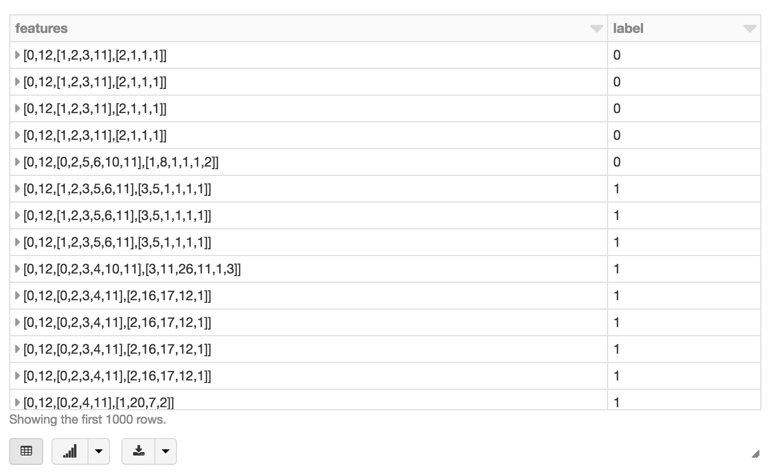
Next, we will split our featurized dataset into training and test datasets via .randomSplit().
train, test = features \
  .select(["label", "features"]) \
  .randomSplit([0.7, 0.3], 42)
Next, we will train, predict, and evaluate our model using the GBTClassifier. As a side note, a good primer on solving binary classification problems with Spark MLlib is Susan Li’s Machine Learning with PySpark and MLlib — Solving a Binary Classification Problem.
from pyspark.ml.classification import GBTClassifier

# Train our GBTClassifier model
classifier = GBTClassifier(labelCol="label", featuresCol="features", maxBins=maxBins, maxDepth=10, maxIter=10)
model = classifier.fit(train)

# Execute our predictions
predictions = model.transform(test)


# Evaluate our GBTClassifier model using
#   BinaryClassificationEvaluator()
from pyspark.ml.evaluation import BinaryClassificationEvaluator
ev = BinaryClassificationEvaluator( \\
rawPredictionCol="rawPrediction", metricName="areaUnderROC")
print ev.evaluate(predictions)

# Output
0.7112027059
With our predictions, we can evaluate the model according to some evaluation metric, for example, area under the ROC curve, and view features by importance. We can also see the AUC value which in this case is 0.7112027059.
Summary
We demonstrated how you can simplify your advertising analytics – including click prediction – using the Databricks Unified Analytics Platform (UAP). With Databricks UAP, we were quickly able to execute our three components for click prediction: ETL, data exploration, and machine learning. We’ve illustrated how you can run our advanced analytics workflow of ETL, analysis, and machine learning pipelines all within a few Databricks notebook.
By removing the data engineering complexities commonly associated with such data pipelines with the Databricks Unified Analytics Platform, this allows different sets of users i.e. data engineers, data analysts, and data scientists to easily work together. Try out this notebook series in Databricks today!
--
Try Databricks for free. Get started today.
The post Simplify Advertising Analytics Click Prediction with Databricks Unified Analytics Platform appeared first on Databricks.
No comments:
Post a Comment