Friday, 24 August 2018
Download Windows 95 as a Windows, Mac, or Linux App, Because You Can

What Do Those Confusing Light Bulb Codes Mean?
The Best Volume-Limiting Headphones for Kids

When it comes to picking a set of headphone for your little one, the qualifications are a bit different than looking for yourself.
Click Here to Continue Reading
Thursday, 23 August 2018
Geek Trivia: The Only Internal Organ In The Human Body Capable Of Regeneration Is The?
What’s new in Hortonworks DataFlow (HDF) 3.2?
Hortonworks DataFlow (HDF) 3.2 was made generally available to our customers on Aug 13th 2018. HDF 3.2 includes the following major innovations and enhancements: HDF and Hortonworks Data Platform (HDP) in the same ecosystem HDF and HDP can now be run in the same ecosystem. This means that HDF and HDP can be managed using […]
The post What’s new in Hortonworks DataFlow (HDF) 3.2? appeared first on Hortonworks.
How to Use MLflow to Experiment a Keras Network Model: Binary Classification for Movie Reviews
In the last blog post, we demonstrated the ease with which you can get started with MLflow, an open-source platform to manage machine learning lifecycle. In particular, we illustrated a simple Keras/TensorFlow model using MLflow and PyCharm. This time we explore a binary classification Keras network model. Using MLflow’s Tracking APIs, we will track metrics—accuracy and loss–during training and validation from runs between baseline and experimental models. As before we will use PyCharm and localhost to run all experiments.
Binary Classification for IMDB Movie Reviews
Binary classification is a common machine learning problem, where you want to categorize the outcome into two distinct classes, especially for sentiment classification. For this example, we will classify movie reviews into “positive” or “negative” reviews, by examining review’s text content for occurance of common words that express an emotion.
Borrowed primarily from François Chollet’s “Deep Learning with Python”, the Keras network example code has been modularized and modified to constitute as an MLFlow project and incorporate the MLflow Tracking API to log parameters, metrics, and artifacts.
Methodology and Experiments
The Internet Movie Database (IMDB) comes packaged with Keras; it is a set of 50,000 popular movies, split into 25,000 reviews for training and 25,000 for validation, with an even distribution of “positive” and “negative” sentiments. We will use this dataset for training and validating our a model.
By simple data preparation, we can convert this data into tensors, as numpy arrays, for our Keras neural network model to process. (The code for reading and preparing data is in the module: data_utils_nn.py.)
We will create two Keras neural network models—baseline and experimental—and train them on our dataset. While the baseline model will remain constant, we will experiment with the two experimental models, by supplying different tuning parameters and loss functions to compare the results.
This is where MLflow’s tracking component immensely helps us evaluate which of the myriad tunning parameters produce the best metrics in our models. Let’s first examine the baseline model.
Baseline Model: Keras Neural Network Performance
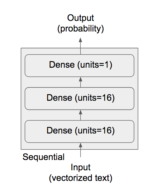
source : Deep Learning with Python
François’s code example employs this Keras network architectural choice for binary classification. It comprises of three Dense layers: one hidden layer (16 units), one input layer (16 units), and one output layer (1 unit), as show in the diagram. “A hidden unit is a dimension in the representation space of the layer,” Chollet writes, where 16 is adequate for this problem space; for complex problems, like image classification, we can always bump up the units or add hidden layers to experiment and observe its effect on accuracy and loss metrics (which we shall do in the experiments below).
While the input and hidden layers use relu as an activation function, the final output layer uses sigmoid, to squash its results into probabilities between [0, 1]. Anything closer to 1 suggests positive, while something below 0.5 can indicate negative.
With this recommended baseline architecture, we train our base model and log all the parameters, metrics, and artifacts. This snippet code, from module models_nn.py, creates a stack of dense layers as depicted in the diagram above.
....
def build_basic_model(self):
 base_model = models.Sequential()
 base_model.add(layers.Dense(16, activation='relu', input_shape=(10000,)))
 base_model.add(layers.Dense(16, activation='relu'))
 base_model.add(layers.Dense(1, activation='sigmoid'))

 return base_model
Next, after building the model, we compile the model, with appropriate loss function and optimizers. Since we are expecting probabilities as our final output, the recommended loss function for binary classification is binary_crosstropy and the corresponding suggested optimizer is rmsprop. The code snippet from module train_nn.py compiles our model.
from keras import optimizers
 ...
 ...
if optimizer == 'rmsprop':
   opt = optimizers.RMSprop(lr=lr)
model.compile(optimizer=opt, loss=’binary_crossentropy’, metrics=[‘accuracy’])
...
Finally, we fit (train) and evaluate by running iterations or epochs with a default batch size for 512 samples from the IMDB data set for each iteration, with default parameters:
- Epochs = 20
- Loss = binary_misantropy
- Units = 16
- Hidden Layers = 1
To run from the command line, cd to the Git repository directory keras/imdbclassifier and run either:
python main_nn.py
Or from the GitHub repo top level directory run:
mlflow run keras/imdbclassifier -e main
Or directly from Gitbub:
mlflow run 'git@github.com:dmatrix/jsd-mlflow-examples.git#keras/imdbclassifier'
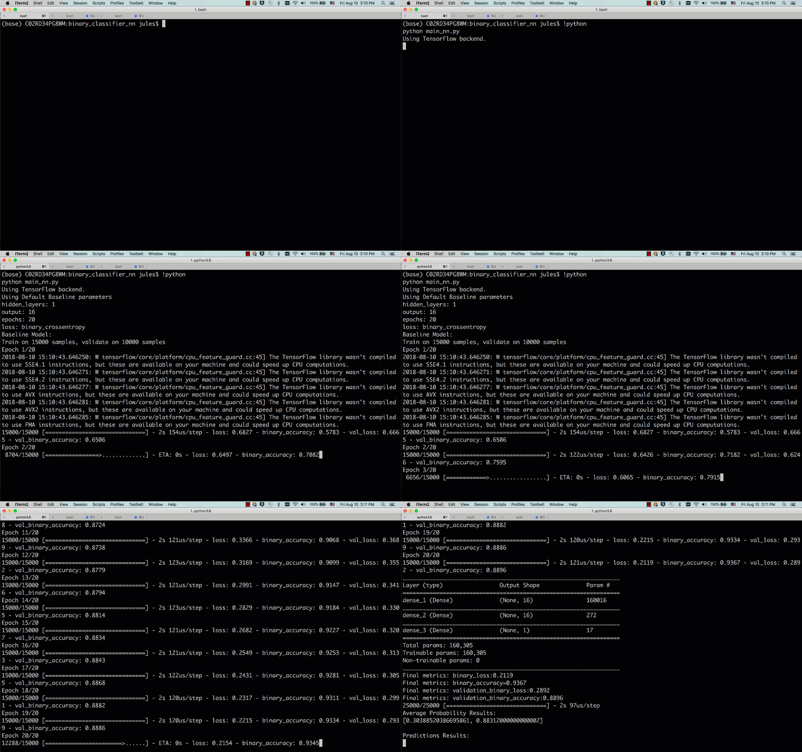
Fig 1: Animated run with base model parameters on a local host
At the end of the run, the model will print a set of final metrics such as binary_loss, binary_accuracy, validation_loss, and validation_accuracy for both training set and validation set after all iterations.
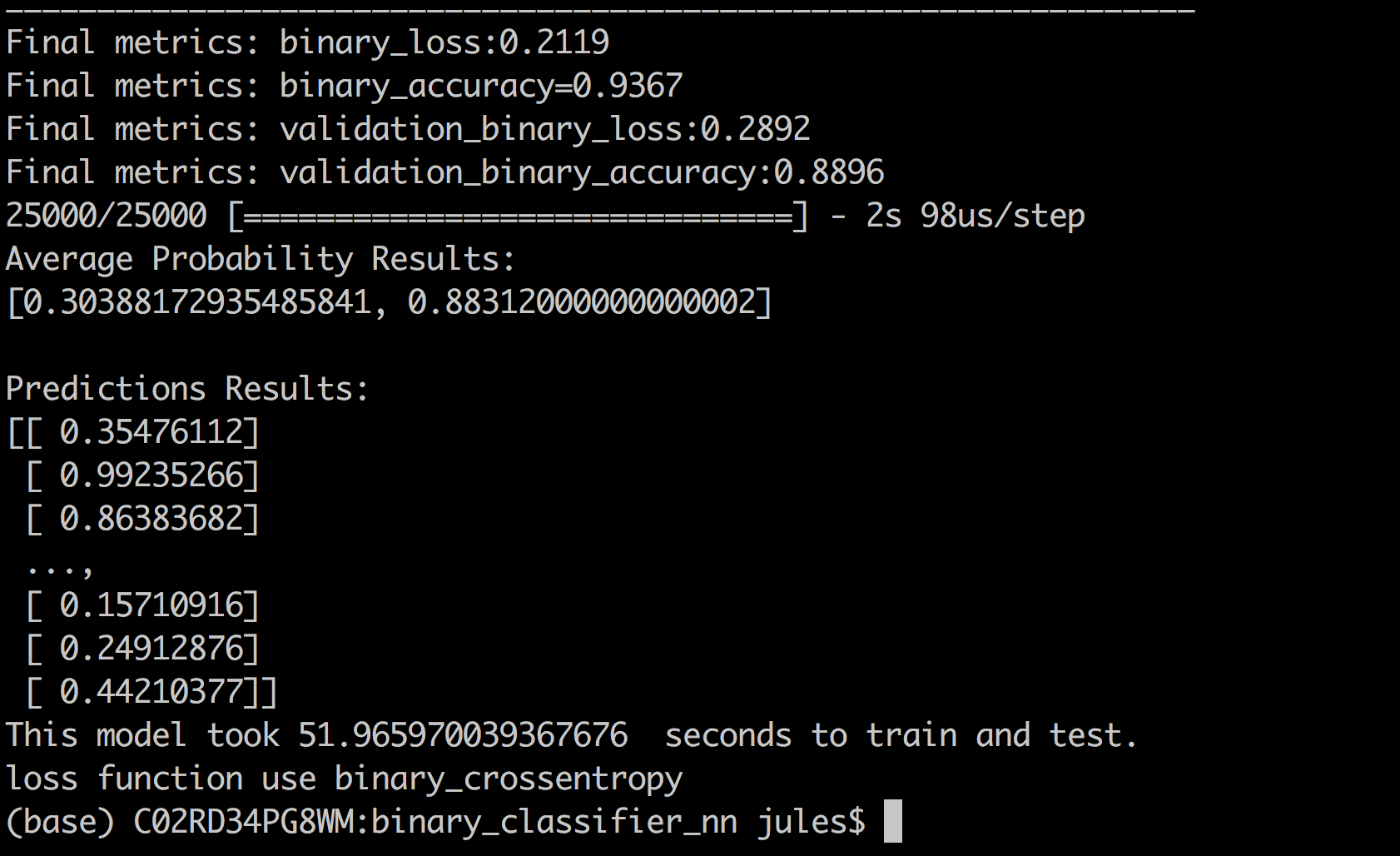
Fig 2: Results and metrics run with base model parameters
As you will notice from the runs, the loss decreases over iterations while the accuracy increases, with the former converging toward 0 and the latter toward 1.
Our final training data (binary_loss) converged to 0.211 and the validation data (validation_loss) tracked with 0.29—which tracked somewhat closely with binary_loss. On the other hand, the accuracy diverged after several epochs suggesting we may be overfitting with the training data (see plots below).
(Note: To access these plots, launch the MLFlow UI, click on any experimental run, and access its artifacts’ folder.)
When predicting with unseen IMDB reviews, the prediction results averaged at 0.88 accuracy, which is close to our validation accuracy, but still fairly far off. However, as you can see, for some reviews the network confidently predicted results with 99% probability of a positive review.
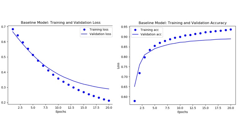
Fig 3a: Matplotlib artifacts logged with base and experiment model parameters
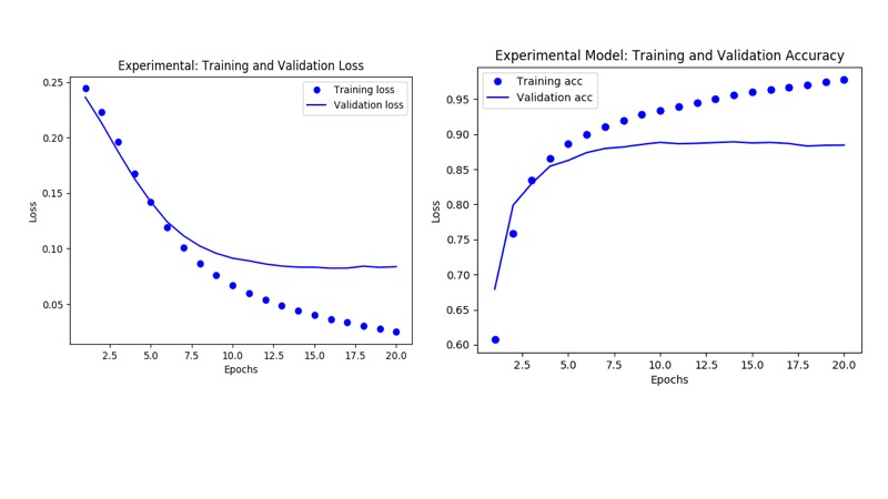
Fig 3b: Matplotlib artifacts logged with base and experiment model parameters
At this point, after observing the basic model metrics, you may ask, can we do better? Can we tweak some tuning parameters such as number of hidden layers, epochs, loss function or units to affect better results. Let’s try with some recommended experiments.
Experimental Model: Keras Neural Network Performance
MLflow’s Tracking Component allows us to track experimental runs of our model with different parameters and persist their metrics and artifacts for analysis. Let’s launch a couple of runs with the following experimental parameters, as Chollet suggests, that are different from the default model and observe an outcome:
| Model | Units | Epochs | Loss Function | Hidden Layers |
|---|---|---|---|---|
| Base | 16 | 20 | binary_crosstropy | 1 |
| Experiment-1 | 32 | 30 | binary_crosstropy | 3 |
| Experiment-2 | 32 | 20 | mse | 3 |
Table 1: Models and Parameters
Running Experiments on Local Host
Since we are running MLflow on the local machine, all results are logged locally. However, you can as easily log metrics remotely on a hosted tracking server in Databricks, by simply setting an environment variable MLFLOW_TRACKING_URI or programmatically set with mlflow.set_tracking_uri().
Either connects to a tracking URI and log results. In both cases, the URI can either be a HTTP/HTTPS URI for a remote server, or a local path to a directory. On the local host, the URI defaults to an mlruns directory.
Running Experiments within PyCharm with MLFlow
Since I prefer PyCharm for my Python development, I’ll run my experiments from within PyCharm on my laptop, providing the experimental parameters. Below is an animation from the first experiment. (To learn how to use MLflow within PyCharm read my previous blog).
Although I ran the experiments by providing parameters within PyCharm’s run configurations, you can just as easily run these experiments on the command line from the top level directory, too:
mlflow run keras/imdbclassifier -e main -P hidden_layers=3 -P epochs=30
mlflow run keras/imdbclassifier -e main -P hidden_layers=3 -P output=32 -P loss=mse

Fig 4: Animated run with experiment-1 model parameters
All experiments’ runs are logged, and we can examine each metric and compare various runs to assess results. All the code that logs these artifacts using MLflow Tracking API is in the train_nn.py module. Here is a partial code snippet:
        ....
        with mlflow.start_run():
            # log parameters
            mlflow.log_param("hidden_layers", args.hidden_layers)
            mlflow.log_param("output", args.output)
            mlflow.log_param("epochs", args.epochs)
            mlflow.log_param("loss_function", args.loss)
            # log metrics
            mlflow.log_metric("binary_loss", ktrain_cls.get_binary_loss(history))
            mlflow.log_metric("binary_acc",  ktrain_cls.get_binary_acc(history))
            mlflow.log_metric("validation_loss", ktrain_cls.get_binary_loss(history))
            mlflow.log_metric("validation_acc", ktrain_cls.get_validation_acc(history))
            mlflow.log_metric("average_loss", results[0])
            mlflow.log_metric("average_acc", results[1])

            # log artifacts (matplotlib images for loss/accuracy)
            mlflow.log_artifacts(image_dir)
          #log model
            mlflow.keras.log_model(keras_model, model_dir)

        print("loss function use", args.loss)

if __name__ == '__main__':
    #
    # main used for testing the functions
    #
    parser = KParseArgs()
    args = parser.parse_args()

    flag = len(sys.argv) == 1

    if flag:
        print("Using Default Baseline parameters")
    else:
        print("Using Experimental parameters")

    print("hidden_layers:", args.hidden_layers)
    print("output:", args.output)
    print("epochs:", args.epochs)
    print("loss:", args.loss)
    train_models_cls = KTrain().train_models(args, flag)
Comparing Experiments and Results with MLFlow UI
Now the best part. MLflow allows you to view all your runs and logged results from an MLflow GUI, where you can compare all three runs’ metrics. Recent UI improvements in MLFlow v0.5.0 offer a better experience in comparing runs.
To launch a Flask tracking server on your localhost:5000, use command line mlflow ui.
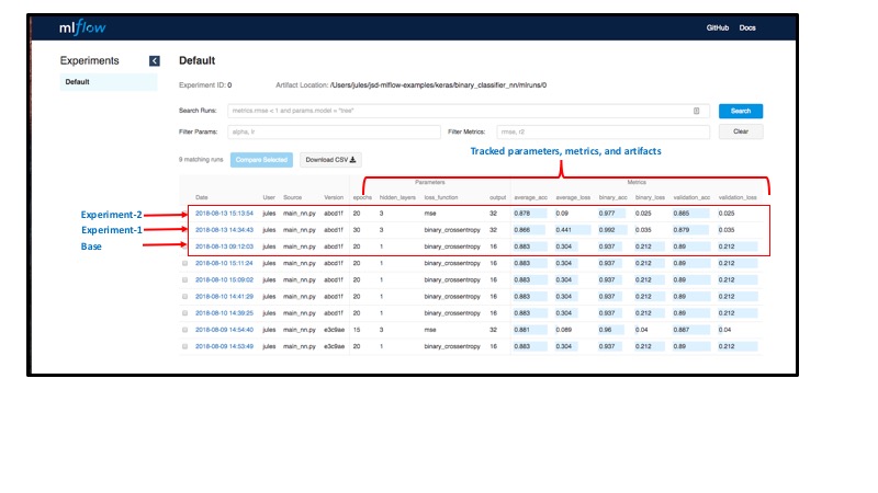
Fig 5: MLflow UI table view of all runs’ metrics, parameters, and artifacts
For example, I can compare all three experiments’ metrics to see which of the runs produced an acceptable validation accuracy and loss as well view each of my experiments’ matplotlib images to see how they fared across epochs.
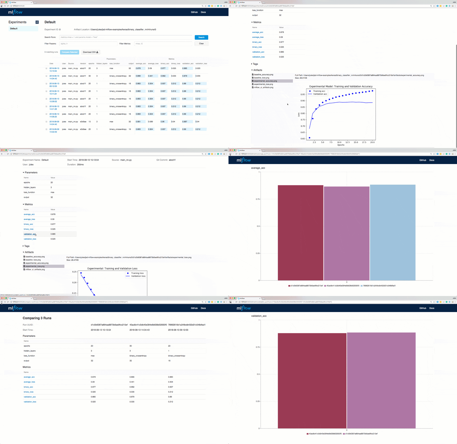
Fig 6: Animated view of metrics with experimental parameters
Comparing Results from Three Runs
By quickly examining our runs in MLFlow UI, we can easily observe the following:
- Changing the number of epochs did not give us any benefit except the model began overfitting, as it reached training accuracy of 99%, with no corresponding difference to validation accuracy, which diverges after several epochs.
- Changing the loss function to
mse, units to 32, and hidden layers to 3, however, gave us a better validation loss as well as a converging average_loss to 0 for the validation data. With other metrics tracking closely across models, a couple of extra hidden layers and more units minimized the validation loss.
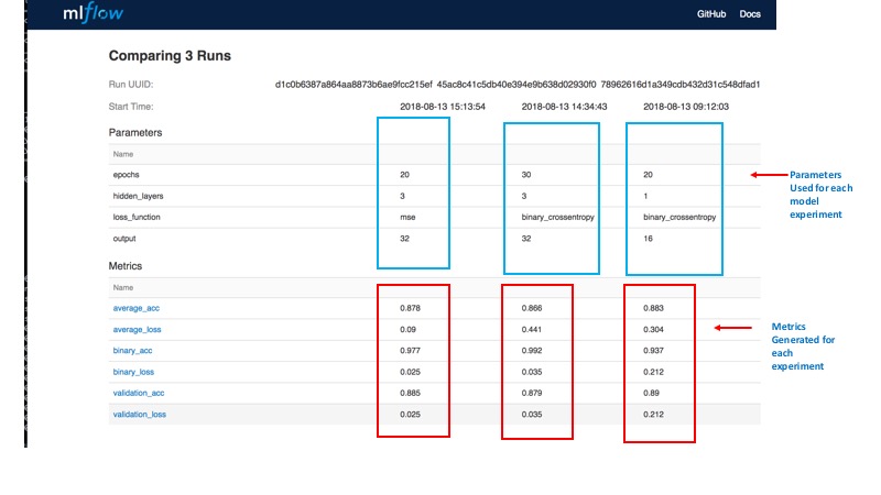
Fig 7: Comparing three run with parameters
Improving Model Metrics With Further Experiments
Notably, François Chollet posits that with further training, validation, and tests (TVT), we can achieve higher accuracy, over 95% and converge the loss to 0.01%. One way to achieve it is through further experiments with machine learning techniques such as
add more data, simple-hold out validation, k-fold validation, add weight regularization, add dropout network layers, and increase network capacity. These could minimize overfitting and achieve generalization—and as consequence drive better accuracy and minimal loss.
We could implement these techniques here, carry out further experiments, and use MLflow to assess outcomes. I’ll leave that as an exercise for the reader.
Because such experiments and iterations are so central to the way data scientists asses models, MLflow facilitates such lifecycle tasks. To that extent, this blog demonstrated that part of MLflow’s functionality.
Closing Thoughts
So far we demonstrated the key use of MLflow Tracking Component’s APIs to log model’s myriad parameters, metrics, and artifacts so that at any point or anyone can reproduce the results from model’s MLflow Git project repository.
Second, through command line, PyCharm runs, and MLFlow UI, we compared various runs to examine the best metrics, and observed that by altering some parameters, we approached a model that could perhaps be used with acceptable accuracy for doing sentiment classification of IMDB movie reviews based on common words that express positive or negative review. Even better, as noted, we could further improve our models’ outcomes by using suggested machine learning techniques.
Finally, but far importantly, we experimented using MLflow within PyCharm on a local host, but we could just as easily track experiments on a remote server. With MLflow, Numpy, Pandas, Keras, and TensorFlow packages installed as part of our PyCharm Python Virtual Environment, this methodical iteration of model experiments is a vital step in a machine learning model’s life cycle. And the MLflow platform facilitates this crucial step—all from within your favorite Python IDE.
What’s Next
Now that we have compared the baseline model to a couple of experimental models and we have seen MLflow’s merits, what is the next step? Try MLflow at mlflow.org to get started. Or try some of tutorials and examples in the documentation.
Read More
Here are some resources for you to learn more:
- Read MLflow Docs
- Find out How to Use Keras, TensorFlow, and MLflow with PyCharm
- Learn from Introducing mlflow-apps: A Repository of Sample Applications for MLflow
- View MLflow Meetup Presentations and Slides
- Get Github sources for this blog example
- Find out New Features in MLflow Release v0.5.0
--
Try Databricks for free. Get started today.
The post How to Use MLflow to Experiment a Keras Network Model: Binary Classification for Movie Reviews appeared first on Databricks.
Facebook Removed Their Spying VPN From The App Store (But It’s Still on Google Play)
Would You Pay a Monthly Fee to Buy An Xbox Over Two Years Like a Cell Phone?

When you go to your cell carrier, they’ll give you an expensive phone up front and let you pay monthly for it for two years.
Click Here to Continue Reading
8 Must Have Products For Your Dorm Room

If you’re heading off to college in the Fall, you’ve probably got a lot of planning ahead of you.
Click Here to Continue Reading
How to Position Images and Other Objects in Microsoft Word
Introducing Hortonworks Streams Messaging Manager (SMM)
Last week, we discussed how the omnipresence of Kafka in application architectures has led to the Kafka Blindness afflicting DevOps/AppDev, Platform Operations and Security/Goverenance teams within the enterprise. These groups are struggling to effectively battle this blindness with the current tooling available. Over the last 12 months, the Hortonworks team has been working with these […]
The post Introducing Hortonworks Streams Messaging Manager (SMM) appeared first on Hortonworks.
What Is a DAT File (and How Do I Open One)?
How to Juggle Multiple Google Calendars
Is It Better to Watch a 4K Movie On Blu-ray or Through Streaming?

Netflix offers 4K movies, but are they good enough to compete with the UHD Blu-ray you can find in a store? Well, no.
Click Here to Continue Reading
What is ZSH, and Why Should You Use It Instead of Bash?
What Does Real-Time Ray Tracing Mean for Gamers Today?
The Complete History of Mac OS X, In Screenshots
8 Good Paid Mobile Games with No Pesky In-App Purchases
Seven Exclusive Nintendo Switch Games Worth Pre-Ordering From Amazon While You Still Can

Nintendo’s got a bunch of games coming down the pipeline, but Amazon is getting rid of its 20% discount before they arrive.
Click Here to Continue Reading
Wednesday, 22 August 2018
Geek Trivia: Johnny Appleseed’s Goal In Planting Apple Trees Was To?
Monument Valley Is Getting Its Own Movie Under Paramount Pictures

You know that cute puzzle game Monument Valley with the faceless protagonist that you played for a few minutes every day for a while?…
Click Here to Continue Reading
Linux Steam Beta Offers Windows Games Using a Compatibility Layer

IKEA Planning a $10 Smart Plug Compatible with HomeKit, Google Assistant, and Alexa
How to Tell How Long You’ve Worked on a Microsoft Word Document
Streamlining the Next-Generation of Genomic Sequencing – Saving Time and Saving Lives
We’ve just published our most recent case study! This story gives an in-depth look at how Quanam is leveraging a modern data architecture along with machine learning, to better equip clinicians. Founded in Uruguay in 1978, Quanam is a multi-Latin federation of firms specializing in consulting and management, professional services, communication and change management. Priding itself on […]
The post Streamlining the Next-Generation of Genomic Sequencing – Saving Time and Saving Lives appeared first on Hortonworks.
