Traffic Mix and AI Autonomous Cars

By Lance Eliot, the AI Trends Insider

Car traffic can be downright exasperating, frustrating, beguiling, exhausting, and just a real pain in the keister (pardon my language).

Most of us dread getting stuck in traffic.

Endless sea of cars.

Stop and go movement.

Bumper to bumper with a chance of some scrapes and fender benders.

There are the looky-loos that aren’t paying attention to the driving task and instead are looking at billboards or watching cows out in the fields (well, for more out-of-the-way driving locales). There are the drivers that seem to think that if they get within an inch of your bumper, it will somehow make the traffic go faster. There are the knuckleheads that have their blinker on for miles at a time, apparently oblivious to the aspect that they are confusing other drivers and causing the rest of us to wonder if the dolt will suddenly change lanes without any actual viable notification.

Many of us bemoan that it’s not us that makes the traffic especially arduous, but instead those other drivers that seem out-of-touch or otherwise confused about how to properly drive in a traffic oriented situation.

Normally, if the traffic is flowing smoothly, there are less of these disruptive drivers or at least they seem less apparent. Once the traffic starts to get clogged, it becomes a real survival-of-the-fittest world. Cars will swing into and out of lanes to try and get a few feet ahead of other cars. Drivers will raise a finger at another driver that appears to cut them off or try to jam into the lane ahead of them. In some cases, things can escalate out-of-hand and produce road rage with at times deadly consequences.

For my article about road rage and AI self-driving cars, please see: https://aitrends.com/selfdrivingcars/road-rage-and-ai-self-driving-cars/

Traffic Is A Delicate Dance Of Cars And Car Driving

Generally, our existing laws and rules-of-the-road allow for human drivers to exercise a certain amount of discretion within loosely bounded legal rules.

When a car to my right suddenly jams into my lane, and fails to signal, and fails to wait until there’s a reasonable opening, and fails to clear my car by more than a fraction of an inch, you could say that they have violated the law by creating an unsafe driving situation. But, who’s going to give them a ticket or stop them from this kind of discretionary driving? Unless by a stroke of luck there’s a traffic cop there, this kind of driving behavior is going to be gotten away with, unfortunately.

Thus, the day-to-day traffic that we survive in can be characterized as not being uniform, and not necessarily enforceable as to the strict interpretation of the laws of driving, and overall allows for human judgement to be used to decide in what way someone will drive their car.

Obviously, if the wayward drivers go beyond the allowed norm, and bash into another car, or they ram into a fire hydrant, or do anything of an “extraordinary” nature that’s a demonstrative law breaker action, the odds are they’ll get caught. I’m here trying to point out that at a level of driving just below that kind of clear cut legal outlaw stage, there is a lot of discretion as to how we can drive our cars.

If the roadway is pretty wide open and there are lots of lanes to choose among, the probability of a wayward discretionary driver that wanders up toward the legal outlaw line and getting caught is relatively low, while once there is a significant amount of traffic the probability generally gets higher. Also, once there is a significant amount of traffic, we now have more cars to contend with, and thus if say only 10% of drivers are the outlaw types, when you have just 10 cars nearby that means there is only 1 driver of the wayward type, while if you have 50 cars then you have 5 that are entered into the mix. In essence, volume of traffic makes a difference.

With the volume of traffic, we also need to consider density.

Generally, the more volume and the higher the density of traffic, the more that the actions of one driver can impact the other cars and drivers.

I realize this is not always true, in the sense that if you have a crazy driver even in light traffic situations, they can readily decide to weave in and around the other few cars and purposely try to cause them to hit their brakes or make other escaping maneuvers. It seems though that more often than not, the lighter traffic tends to allow for wayward drivers to do their thing without having as much a disruptive influence.

We could say that this is perhaps due to the magnitude of coupling.

Cars that have lots of room around themselves to maneuver can be considered more loosely coupled to those other cars around them. When the space between cars is tightened, it tends to increase coupling. I am referring to a virtual kind of coupling, and not any kind of true physical connections. It’s as though we had virtual invisible elastic bands that are connecting the nearby cars, and so when there is plenty of room then the cars are remotely coupled, and when they are closer to each other they are more directly coupled.

In close quarters traffic, if you suddenly get in front of my car by switching lanes without warning, and you do so within feet of my front bumper, I am likely to touch on my brakes to give you some added room and try to ensure that I don’t ram into the back of your car. Meanwhile, the car behind me, which we’ll say is also in close quarters, they too now might need to touch on their brakes. And so on it goes. A cascading effort can occur. It’s like a bunch of dominos lined up.

If it wasn’t close quarters traffic, and I touched my brakes, the car behind me which let’s say in this circumstance is some distance behind me, might not need to touch on their brakes. Instead, via the natural flow of traffic, they might be able to come a little closer and then we are still moving along freely. When the density of the traffic increase, which usually is also associated with the volume of traffic, the coupling aspects tend to mean that whatever happens with one car can cascade into other cars. Again, think of dominoes, but if they are spread out then when one falls it doesn’t necessarily cause the other one to fall too.

There are times that I’ve been on the open highway and had a high density of traffic, even though the volume of traffic was low.

A clump of cars happened to all get close to each other, even though the highway had miles upon miles of open space ahead of and behind us. This clumping can occur on a momentary basis, after which the cars then disperse out into the available open space. Or, sometimes the clump can remain a clump. This can be frustrating if you are part of the clump and don’t want to be in it. You’ve perhaps had to slow down demonstrably to let the pack move ahead, or maybe you’ve sped up mightily to get way beyond the pack.

Some drivers don’t seem to recognize when they’ve gotten themselves into such a clump.

They are just keeping their noses down and staring at the car ahead of them. Several of these cars with the heads-down kind of driver can eventually can meet up. They become a clump, basically by default. Not one of them thinks to get out of the clump. Other cars come along, encounter the clump, and at times get stuck in the clump as well. It can be difficult to get around a clump and might take numerous adroit attempts to do so.

The driving leapfrog techniques often applies when there are clumps, see my article on leapfrogging and AI self-driving cars:  https://aitrends.com/selfdrivingcars/leap-frog-driving-self-driving-cars/

AI Autonomous Cars And Traffic Mix

What does this discussion about traffic mix have to do with AI self-driving driverless autonomous cars?

At the Cybernetic Self-Driving Car Institute, we are developing AI systems for self-driving cars and have been studying extensively traffic mix and the nature of self-driving car driving techniques and approaches.

Some AI pundits claim that there’s no need to study traffic mix since the world will be a wondrous place once we have all self-driving cars on the roadways.

In this Utopia, the self-driving cars will all communicate with each other via V2V (vehicle-to-vehicle communication), and politely share the roads with each other. An AI self-driving car will convey to another one that it wants to please go ahead and get into the lane with that one, and the responding AI self-driving car will communicate that yes, please do. They will dance together in a coordinated and cooperative manner. Furthermore, with the use of V2I (vehicle-to-infrastructure communication), these AI self-driving cars will be informed by the roadway that there’s a bump in the road up ahead, and the AI self-driving cars will ready themselves to handle the bump.

Nice!

This might someday be our future.

But, until then, the real truth of the matter is that we’re going to have a mixture of AI self-driving cars and human driven cars. I say this because right now in the United States alone we have about 200+ million conventional cars. Those conventional cars aren’t going to disappear overnight. Instead, it will be years upon years, more like decades, before we gradually see AI self-driving cars becoming widespread and overtaking the number of human driven cars. Eventually, it may be that there are no human-driven cars, or it could be that people will insist on still being able to drive a car.

AI pundits complain that if humans still insist on driving a car, it’s going to mess things up. In one sense, they might be right. Based on studying the nature of traffic mixes, we can simulate what the future might be like in terms of the mix of human driven cars and AI self-driving cars.

Let’s first start by thinking about proportions related to the mix:

• 1:N – this is one AI self-driving car that is in the midst of N human driven cars
• N:1 – this is N number of AI self-driving cars that are in the midst of one human driven car
• 10%:N – this is a ten percentage mix of AI self-driving cars in a volume of cars that includes N human driven cars
• 30%:70% — this is a circumstance wherein the volume of cars has 30% that are AI self-driving cars and has 70% that are human driven cars
• Etc.

I’ll be using this above nomenclature when referring to the various mixtures in traffic of AI self-driving car and human driven cars.

Let’s also agree that when I refer to a volume of traffic, it is with respect to a given circumstance.

I am also going to for now make the assumption that we have a relatively high density of traffic in these circumstances and the volume is relatively high too. I mention this for the same reasons that I had earlier stated that when the traffic is wide open, the nature of how the traffic intermixes is generally different than the circumstances when there is tighter coupling.

We also need to agree what we mean by an AI self-driving car.

Herein, I’m going to refer to an AI self-driving car as one that is at the Level 4 and Level 5, which are the levels at which the AI self-driving car is considered the driver of the car, and does not need a human driver, and can drive in whatever manner a human driver can drive. Levels less than 4 involve having a human driver available in the AI self-driving car, doing so in case the human driver needs to take over the driving task or is given the driving task from the AI.

It’s important to consider that these traffic mix simulations involve a Level 4 and Level 5 self-driving car. For simulations with less than a Level 4, you would need to also include aspects of the human driver that might take over the control of the self-driving car. This would definitely impact the nature of how the AI self-driving car is going to be reacting in the simulation since you’d need to account for the times when the human driver is driving the self-driving car versus the AI is driving the self-driving car.

Another factor to consider involves the sophistication of the AI self-driving car. Even once we get to the Level 4 and Level 5, there are going to be proficient AI self-driving cars at those levels and others that we could reasonably agree aren’t as proficient. Not all of the Level 4 and Level 5 rated AI self-driving cars will necessarily be at the same level of driving skills.

Over time, there will be ongoing and continued improvements in the driving skills of even the Level 4 and Level 5 self-driving cars.

See my article about the defensive driving tactics of AI self-driving cars: https://aitrends.com/selfdrivingcars/art-defensive-driving-key-self-driving-car-success/

Additional Factors To Be Considered

There are more factors to be considered too about the traffic mix situation.

One really vital question involves how will human drivers react to AI self-driving cars?

You might at first say that human drivers won’t react any differently to an AI self-driving car than they do to another human driven car.

Well, you’d be wrong.

Human drivers will definitely be reacting differently to AI self-driving cars than they do to human driven cars, at least for the foreseeable future.

We’ve already seen that when AI self-driving cars are among conventional human traffic, the human drivers tend to give the AI self-driving car wide berth. It’s as though the human drivers consider the AI self-driving car to be the equivalent of a novice teenager learning to drive. The human drivers are suspicious of the capabilities of the AI self-driving car. The human drivers are wary that the AI self-driving car might make an odd maneuver or do something untoward. Thus, human drivers opt to treat the AI self-driving car differently than a normal everyday human driven car.

You might object and say that the human drivers won’t even necessarily be aware that another car around them so happens to be an AI self-driving car.

I disagree.

Right now, the experimental AI self-driving cars on the roadway are at times rather obviously detected, since there are only certain brands of cars right now that are outfitted as self-driving cars. Also, noticeably absent is any driver in the driver’s seat. Plus, some of the self-driving cars today have a LIDAR device on the roof of the car, and some also have branding on the sides of the self-driving car to point out that they are self-driving cars.

It is also relatively easy to detect today’s self-driving cars by the manner in which they drive.

Most of them are driving very slowly and cautiously. They come to a full stop at stop signs. They go less than the speed limit in places that most human drivers exceed the speed limit. They timidly proceed when an intersection light goes green. I realize that some human drivers also drive this way, but I am just saying that when you combine the driving behavior of today’s AI self-driving cars with the other more physically apparent aspects, you can generally know when you are driving next to or near a self-driving car.

This is a crucial factor when creating a simulation.

Most of the traffic mix simulations assume that the human drivers will be unaware that they are driving with AI self-driving cars around them. The simulations also assume that the AI self-driving car will drive in the same manner that humans drive cars, such as speeding, cutting corners, and so on.

Or, worse still, the simulations assume that all drivers will all abide strictly by the rules of driving and be polite and respectful, regardless whether a human driver or an AI self-driving car. I think we can agree that human drivers don’t drive that way.

Therefore, a realistic traffic mix simulation needs to consider for now that:

• Human drivers will drive as human drivers do, exploiting their allowed latitude and being wayward
• AI self-driving cars for the foreseeable future will drive in a more limited novice manner and be hardly wayward at all
• Human drivers will drive differently upon detecting that an AI self-driving car is nearby and will re-actively drive because of the AI self-driving car being in their midst

Maybe, far in the future, human drivers will become accustomed to driving around AI self-driving cars and so they won’t think twice about it.

Likewise, perhaps in the future the AI self-driving cars will drive more akin to how humans drive, doing so with a bit of swagger.

Traffic Mix Proportions

Let’s now return to the traffic mix proportions.

An interesting research study seems to suggest that having even one AI self-driving car, equipped with V2V, could improve safety and save energy in traffic (a study at the University of Michigan, “Experimental Validation of Connected Automated Vehicle Design Among Human-Driven Vehicles,” partially funded by Mcity).

I applaud the researchers for their efforts.

Not only did they do simulated aspects, they also ran a series of experiments on public roadways with actual cars, including AI self-driving cars and human driven cars.

This is the kind of work needed to help advance the AI self-driving car emergence.

In the experiment, the researchers were exploring what happens in a chain of cars when there is a cascading impact or chain-reaction due to a car braking and then re-accelerating. They found that the self-driving car was able to more smoothly deal with the circumstance, braking with 60% less of the G-forces and improving energy efficiency by 19%. The humans involved in the driving experiment were acting as a typical human driver might, namely tending to brake hard when caught by surprise about the chain reaction and then having to do a more rapid re-acceleration too.

Part of the trick here in this experiment is the V2V aspects.

This is great, but it also is focused on the future of when we’ll actually have widespread V2V.

Until then, we’re going to have AI self-driving cars on the roadways that either lack V2V, or are outfitted with V2V but no other cars anywhere near them also have V2V.

Also, as stated in their research, they were focused on single lane types of driving, and more expansive studies are needed to look at a fuller mix of traffic including multi-lane situations.

In our simulations, using the aforementioned assumptions about driver behaviors, we’ve found that when you have the situation of 1:N, this tends to actually worsen the traffic situation.

When there is a sole AI self-driving car among many human driven cars, it’s the equivalent of having a novice teenage driver among many seasoned drivers. The novice driver tends to go slowly and react timidly, which then causes the seasoned drivers to become provoked and try to find ways around that driver. It’s like a stream of water that a rock has been tossed into. The rest of the stream tries to find ways to get around that car. This is something to keep in mind in these early days of the adoption of AI self-driving cars on our public roadways.

In a similar kind of result, there’s the N:1.

When you have essentially all AI self-driving cars and mix into it just one human driven car, it tends to disrupt the traffic. This is because the wily human driver tends to drive in a wayward fashion, while the AI self-driving cars are all trying to work cooperatively and in coordination with each other.

Now, I would suggest that we’re not going to see anytime soon an entire array of AI self-driving cars and one lone human driven car mixed together.

By the time that happens, I’m betting that the AI self-driving cars will have been better equipped and programmed to handle the wayward human drivers and so they will be adept enough to cope with the human driver in their midst. In essence, I’m suggesting that by the time there is only a lone human driver among lots of AI self-driving cars, we will likely have first had a more proportionate mix of AI self-driving cars and human driven cars, and when the last few holdout human drivers are around will we have the N:1 circumstance (they’ll have to pry the steering wheel from their cold hard hands, so to speak).

Let’s consider the 30%:70% as an example.

In this case, the simulation consists of a volume of cars in a high density situation that has 30% or about one-third that are AI self-driving cars, and the rest or 70% are human driven cars. What happens in this scenario? Under the same assumptions as earlier stated, the human drivers are now beginning to get used to the AI self-driving cars and adjusting their driving behavior accordingly. The traffic appears to sway toward the AI self-driving car mode of driving. It’s as though the human drivers are now among a sizable bunch of teenage novice drivers, and the seasoned drivers are giving into their way of driving.

We still see traffic waves occurring in this mix.

Until the proportion of AI self-driving cars gets high enough and reaches a threshold, the human driven cars are still generally operating as humans do. With enough of the AI self-driving cars and once they get sophisticated enough, they are able to contend with those disruptive drivers. The disruptive drivers eventually too figure out that the AI self-driving cars are wise to them. Up until that point, the human drivers figure they’ll pull the wool over the eyes of the AI self-driving cars and treat them like patsies that are readily exploitable.

Another aspect that we include in our simulations is the impact of other driving aspects such as the mix of having motorcyclists, pedestrians, bicyclists, and other traffic elements.

Some studies focus on freeway only traffic situations, which then cuts out pedestrians, bicyclists, and other city or street regular driving circumstances. Some AI pundits say that we should have freeways devoted solely to AI self-driving cars, or if that’s not feasible then at least have lanes dedicated to AI self-driving cars. The concept there is that we might be able to gain the advantages of the all-and-only AI self-driving cars by giving them their own place to drive. This though will require some potential hefty changes in our roadway infrastructure.

See my article about induced demand and AI self-driving cars: https://aitrends.com/selfdrivingcars/induced-demand-driven-by-ai-self-driving-cars/

Conclusion

Today’s traffic can be maddening.

Imagine in the future when you get stuck in bumper to bumper traffic and look at the car next to you and there’s no one driving the car.

Will you still be able to show your finger to that non-human self-driving car? Even if you can, will it make a difference?

In whatever manner this all plays out, I think we can assume that we’ll have a small proportion of AI self-driving cars at first, which will gradually grow over time. At each of these stages of evolution of our traffic mix, we’ll see somewhat different traffic patterns emerge.

This is crucial to keep in mind when planning how we’ll be dealing with the mixing together of human drivers and AI self-driving cars.

Will it be like oil and water?

Or, can we get it to be more like milk and cereal?

Copyright 2019 Dr. Lance Eliot

This content is originally posted on AI Trends.

[Ed. Note: For reader’s interested in Dr. Eliot’s ongoing business analyses about the advent of self-driving cars, see his online Forbes column: https://forbes.com/sites/lanceeliot/]

AI Helping Consumers to Gain More Control over Data Permissions

By AI Trends Staff

As AI systems become better and better at crunching data, companies are responding to expanding efforts to guard data privacy by offering consumers more options for granting or withholding permission.

A new generation of customer data platforms (CDPs) is helping this along. A CDP is used to create a persistent, unified customer database accessible to other systems. Its data is pulled from multiple sources, cleaned, and combined to create a single customer profile.

The process of populating the CDP builds a trail tracing where the customer data came from. This is important in the era of the General Data Protection Regulation (GDPR), which went into effect in the European Union in 2018.  Now it is imperative to know from a compliance standpoint whether the customer data came from Europe, North America, or elsewhere, noted a recent article in CMS Wire. The well-managed CDP can help a company stay in compliance.

And it can help to honor the declared preferences of customers about how they wanted to be contacted, thus earning trust for the site owner.

Website operators are preparing for a new law going into effect in California in January 2020, the California Consumer Privacy Act. The new law gives consumers the right to know what type of data an organization has collected on them, how the data is being used, and which third-party organizations are allowed to share the data.

As consumers exert more control over their information, companies need to be more cognizant of where their customer data came from. “First-party” data, collected directly with permission from the customer, will be more highly valued than “third-party” data, based on essentially surveillance of web browsing behavior the company has purchased, suggested the CMSWire authors.

The authors stated, “In this new era of consumer privacy regulations, connecting third-party data with first-party data can be toxic. You’ve now got identifiable information on individuals they didn’t agree to share. Also, the accuracy of third-party data can be questionable.”

At the same time privacy and data permissions are moving to the fore, the major vendors are enhancing their CDP platforms. Recently at its Dreamforce meeting, Salesforce announced its Customer 360 Truth offering, an enhanced set of CDP services to unify user identities, streamline customer profiles, and handle GDPR requirements, according to an account in Forbes.

Microsoft, Oracle, and Adobe are also implementing CDPs to work toward the “360 degree” customer view, pulling in more structured and unstructured data.

This rise of multiple models is likely to slow the standardization drift, suggest the Forbes authors.

Google Treading Carefully on Facial Recognition of Celebrities

The power of AI is causing Google to tread carefully with the availability of a facial recognition service announced in October that identifies celebrities, according to an account in Wired. Microsoft and Amazon launched similar services in 2017.

Google decided to put limits on the strategy after reviewing its compliance with ethics principles the company introduced last year. Tracy Frey, director of strategy at Google’s cloud division, said the company had concerns about making the service broadly available.

Google commissioned a human rights assessment of the new service from BSR, a non-profit committed to helping along “a just and sustainable world.” BSR’s report suggested that celebrity facial recognition could be used intrusively. The firm suggested that Google allow individuals to opt out of the service, and that it evaluate interested parties before giving access to the service.

In response, Google has limited the service to thousands of celebrities in an effort to minimize the risk of abuse. Google has also provided a web form for anyone to ask that their face be removed from the company’s’ watch list. Prospective customers of the service must pass a review.

Frey said awareness of the tension between the power of AI to do good and the potential downsides have caused the company to be wary. As companies make more use of AI, “They’re looking to us for guidance and to see that we are giving them tools they can trust,” Frey stated.

Android 10 Offers More Permission Options

More permission options are also being offered in the recently-released Android 10 operating system for mobile phones. In the past, granting permission in Android had been either a yes or no proposition. In the new version, the user can specify that an app can only access your location data while you are using that app, and not while it’s not being used, according to an account in Digital Trends.

Also, app developers will be encouraged to explain why their app needs permissions. Only 18% of Android users allow apps all the permissions they request, according to the Digital Trends authors. The top reason for denial is that the “app shouldn’t need the permission.”

The trend for consumers to be able to exert more control over how their data is collected and used, is a fortunate development as AI tools and services continue their march to the mainstream.

Trust to Become a Powerful Differentiator

Trust will become a powerful differentiator in the new data economy, suggests Tim Walters, Ph.D., in a new white paper entitled “Promise and Permission: The Role of Trust in the New Data Economy.”

“As consumers assert more control over their data, they will tend to share it with companies that are both reliable data stewards and attractive partners in a mutual exchange of value. In short, the perceived trustworthiness of a company will be the decisive factor that determines whether consumers provide access to personal data. Marketers need to understand and master the dynamics of trust in personal data exchanges,” he states.

The trend for consumers to be able to exert more control over how their data is collected and used, is a fortunate development as AI tools and services continue their march to the mainstream.

Read the source articles mentioned in CMS Wire, Forbes, Wired and Digital Trends.

Researchers Build Framework To Avoid Machine Learning’s “Undesirable Outcomes”

By Benjamin Ross, Senior Editor, AI Trends

Researchers at Stanford and the University of Massachusetts Amherst have introduced a framework for designing machine learning (ML) algorithms that make it easier for potential users to specify safety and fairness constraints. Details of the framework were recently published in Science (DOI: 10.1126/science.aag3311).

According to the paper’s authors, current machine learning algorithms “often exhibit undesirable behavior, from various types of bias to causing financial loss or delaying medical diagnoses.” What’s worse, the burden of avoiding these pitfalls often falls on the user of the algorithm and not the algorithm’s designer.

The framework “allows the user to constrain the behavior of the algorithm more easily, without requiring extensive domain knowledge or additional data analysis,” the author’s write, which shifts the burden of ensuring that the algorithm is well-behaved from the user of the algorithm to the designer of the algorithm.

As machine learning algorithms have an increasing impact on society, the paper’s authors argue it is important to establish safeguards that will prevent these “undesirable outcomes.” If these outcomes can be defined mathematically, both users and the algorithm can learn how to navigate away from them.

In an official statement, Philip Thomas, an assistant professor of computer science at the University of Massachusetts Amherst and first author of the paper, explains that the framework makes it easier to ensure fairness and avoid harm for a wide range of industries. It does so by generating “Seldonian algorithms,” an allusion to Hari Seldon, a fictional character created by science fiction writer Isaac Asimov. In a particular story, Seldon develops an algorithm that allows him to predict the future in probabilistic terms.

Philip Thomas, Assistant Professor Computer Science, UMass Amherst

Thomas writes that the framework is a tool that guides researchers to create algorithms that are easily applied to real-world problems.

“If I use a Seldonian algorithm for diabetes treatment, I can specify that undesirable behavior means dangerously low blood sugar, or hypoglycemia,” Thomas states. “I can say to the machine, ‘while you’re trying to improve the controller in the insulin pump, don’t make changes that would increase the frequency of hypoglycemia.’ Most algorithms don’t give you a way to put this type of constraint on behavior; it wasn’t included in early designs.”

The framework works in three steps. First, it defines the goal for the algorithm design process. Second, it defines the interface that the user will use. Third, the framework creates the algorithm.

In order to show viability, the researchers designed regression, classification, and reinforcement learning algorithms using the framework.

As a test for their framework, the paper’s authors applied generated algorithms to a data set of 43,000 students in Brazil, predicting students’ grade point averages (GPAs) during their first three semesters at university on the basis of their scores on nine entrance exams, using a sample statistic that captures sexism as a form of discrimination.

Results showed that commonly used regression algorithms designed using the standard ML approach can discriminate against female students when applied without considerations for fairness. “In contrast, the user can easily limit the observed sexist behavior… using our Seldonian regression algorithm,” the authors write.

Thomas and his co-authors hope their framework will open up new avenues for ML application.

“Algorithms designed using our framework are not just a replacement for ML algorithms in existing applications,” Thomas and co. write. “It is our hope that they will pave the way for new applications for which the use of ML was previously deemed to be too risky.”

Learn more at Science (DOI: 10.1126/science.aag3311).

Update on AI for Good: Making Business Sense, and a Cautionary Note

By AI Trends Staff

AI for Good is a United Nations platform that fosters a dialogue on the beneficial use of AI by developing concrete projects. Progress is being made in specific areas, public relations around the topic is positive, and a cautionary note was recently sounded by a respected researcher.

IBM launched Science for Social Good in 2016 aiming to apply technology to 17 issues highlighted by the United Nations as Sustainable Development Goals. These included reducing poverty, inequality, and damage to the environment, while raising standards of healthcare and education around the world.

IBM recently announced progress made across 15 of those 17 issues. In a recent account in Forbes, author Bernard Marr reported on interviews with IBM fellow Aleksandra Mojsilovic and principal research Kush Varshnev about the work.

The idea had its genesis in 2013 or so. Then IBM had “3,000 researchers around the world, and we decided there had to be a way to leverage these skills more broadly and in a coherent way… it didn’t seem right that we were trying to solve these problems in our spare time,” Mojsilovic stated in the Forbes article.

Aleksandra Mojsilovic, IBM Fellow, IBM Research AI

IBM learned some lessons fighting the Ebola outbreak of 2014-2016 in West Africa. “We learned that having a program that’s really focused on creating tools or technology won’t work without the participation of those who really work with these problems,” Mojsilovic stated.

Initiatives were subsequently launched to address fairness around risk assessment in financial services, health insurance in the US, and mobile-based money lending programs in east Africa.  The goal was to use technology to mitigate the risk of bias leading to unfair outcomes.

Examples of AI for social good are tracked by McKinsey in an annual report. Under the category of equality and inclusion, one use case was based on the work of Affectiva, spun out of the MIT Media Lab, and Autism Glass, a Stanford research project. The project used AI to automate the recognition of emotions and provide social cues to help individuals on the autism spectrum interact in social situations.

Mwila Kangwa, CEO, AgriPredict of Zambia, a web and mobile-phone-based agricultural risk management platform built on AI and machine learning, participated in the AI for Good Global Summit held in Geneva in May, 2019.  AgriPredict provides farmers with tools to help identify diseases, predict pest infestations and weather conditions. A farmer takes a picture of the suspected diseased plant, and the system provides a diagnosis, options for treatment, and the location of the nearest agro supplier. Farmers can also receive information on weather patterns. Users access the services on smart phone applications and social media including Twitter, Facebook, and Whatsapp. The service can also be accessed via a USSD platform used by cellular telephones for those without a smartphone.

CEO Kangwa told AI Trends, “We are very much active at AgriPredict. We are currently expanding our products and range for crop disease detection.”

A panel on innovative applications of AI in education at the AI for Good Global Summit included representatives of: Minecraft Education, offering an open-world game that promotes creativity, collaboration and problem-solving; and the Connect to Learn public-private partnership from Ericsson, which strives to increase access to quality education, especially for girls, through life skills programs, the integration of technology tools and digital learning resources in schools.

The Chan Zuckerberg Initiative, from Mark Zuckerberg of Facebook and his wife, Priscilla Chan, is engaged in using technology to address a range of challenges including affordable housing. The initiative formed the Partnership for the Bay’s Future. A public-private partnership that aims to protect up to 175,000 households over the next five years, and produce more than 8,000 homes in the next five to 10 years in the Bay Area.

Caution Issued On AI for Good “Beta Testing”

A caution that AI for good projects can often amount to pilot beta testing with unproven technologies, was issued by Mark Latonero in a recent account in Wired. Dr. Latonero is the Research Lead for Human Rights at Data & Society. He is a fellow at Harvard Kennedy School’s Carr Center for Human Rights Policy, Berkeley Law’s Human Rights Center, and USC’s Annenberg Center for Communication Leadership & Policy, where he earned his Ph.D.

Dr. Latonero works on the social and policy implications of emerging technology and examines the benefits, risks, and harms of digital technologies, particularly in human rights and humanitarian contexts.

“Tech companies that set out to develop a tool for the common good, not only their self-interest, soon face a dilemma: They lack the expertise in the intractable social and humanitarian issues facing much of the world,” he stated. Thus, many enter partnerships. IBM’s social good program has 19 partners; Facebook partners with the Red Cross to help find missing people after disasters. “Partnerships are smart. The last thing society needs is for engineers in enclaves like Silicon Valley to deploy AI tools for global problems they know little about,” Latonero stated.

Read the source articles in Forbes, from McKinsey, and in Wired.

AI is the Key to Unlocking Massive Business Growth in 2020

Artificial intelligence is making a major impact on the future of business. In order to understand the benefits of AI in the world of business, it can be good to look at the historical context of AI technology.

Business Owners Set Aside Skepticism of AI

When the movie "Space Odyssey 2001" was released in 1968, the world got a glimpse of what Artificial Intelligence might look like 30 something years later. Hal, the computer, drove fears about how machines could eventually be the downfall of mankind.

Here in 2019, the world has been living for years among machines that have the ability to learn and think. The challenge for mankind has been to move people beyond their fears that were invoked by Hal. It's the only way the ordinary Joe is going to be able to embrace Artificial Intelligence (AI) integration into everyday life.

It was difficult for many business owners to consider the benefits of AI when they only had science fiction movies to use as a basis for their opinion. It is easy to understand why many of them used to overlook its promising opportunities. However, that is changing dramatically in the 21st Century.

In fact, AI like CPQ is proving to be far ...


Read More on Datafloq

Processing Geospatial Data at Scale With Databricks

The evolution and convergence of technology has fueled a vibrant marketplace for timely and accurate geospatial data. Every day billions of handheld and IoT devices along with thousands of airborne and satellite remote sensing platforms generate hundreds of exabytes of location-aware data. This boom of geospatial big data combined with advancements in machine learning is enabling organizations across industry to build new products and capabilities.

Maps leveraging geospatial data are used widely across industry, spanning multiple use cases, including disaster recovery, defense and intel, infrastructure and health services.

For example, numerous companies provide localized drone-based services such as mapping and site inspection (reference Developing for the Intelligent Cloud and Intelligent Edge). Another rapidly growing industry for geospatial data is autonomous vehicles. Startups and established companies alike are amassing large corpuses of highly contextualized geodata from vehicle sensors to deliver the next innovation in self-driving cars (reference Databricks fuels wejo’s ambition to create a mobility data ecosystem). Retailers and government agencies are also looking to make use of their geospatial data. For example, foot-traffic analysis (reference Building Foot-Traffic Insights Dataset) can help determine the best location to open a new store or, in the Public Sector, improve urban planning. Despite all these investments in geospatial data, a number of challenges exist.

Challenges Analyzing Geospatial at Scale

The first challenge involves dealing with scale in streaming and batch applications. The sheer proliferation of geospatial data and the SLAs required by applications overwhelms traditional storage and processing systems. Customer data has been spilling out of existing vertically scaled geo databases into data lakes for many years now due to pressures such as data volume, velocity, storage cost, and strict schema-on-write enforcement. While enterprises have invested in geospatial data, few have the proper technology architecture to prepare these large, complex datasets for downstream analytics. Further, given that scaled data is often required for advanced use cases, the majority of AI-driven initiatives are failing to make it from pilot to production.

Compatibility with various spatial formats poses the second challenge. There are many different specialized geospatial formats established over many decades as well as incidental data sources in which location information may be harvested:

• Vector formats such as GeoJSON, KML, Shapefile, and WKT
• Raster formats such as ESRI Grid, GeoTIFF, JPEG 2000, and NITF
• Navigational standards such as used by AIS and GPS devices
• Geodatabases accessible via JDBC / ODBC connections such as PostgreSQL / PostGIS
• Remote sensor formats from Hyperspectral, Multispectral, Lidar, and Radar platforms
• OGC web standards such as WCS, WFS, WMS, and WMTS
• Geotagged logs, pictures, videos, and social media
• Unstructured data with location references

In this blog post, we give an overview of general approaches to deal with the two main challenges listed above using the Databricks Unified Data Analytics Platform. This is the first part of a series of blog posts on working with large volumes of geospatial data.

Scaling Geospatial Workloads with Databricks

Databricks offers a unified data analytics platform for big data analytics and machine learning used by thousands of customers worldwide. It is powered by Apache Spark™, Delta Lake, and MLflow with a wide ecosystem of third-party and available library integrations. Databricks UDAP delivers enterprise-grade security, support, reliability, and performance at scale for production workloads. Geospatial workloads are typically complex and there is no one library fitting all use cases. While Apache Spark does not offer geospatial Data Types natively, the open source community as well as enterprises have directed much effort to develop spatial libraries, resulting in a sea of options from which to choose.

There are generally three patterns for scaling geospatial operations such as spatial joins or nearest neighbors:

1. Using purpose-built libraries which extend Apache Spark for geospatial analytics. GeoSpark, GeoMesa, GeoTrellis, and Rasterframes are a few of such libraries used by our customers. These frameworks often offer multiple language bindings, have much better scaling and performance than non-formalized approaches, but can also come with a learning curve.
2. Wrapping single-node libraries such as GeoPandas, Geospatial Data Abstraction Library (GDAL), or Java Topology Service (JTS) in ad-hoc user defined functions (UDFs) for processing in a distributed fashion with Spark DataFrames. This is the simplest approach for scaling existing workloads without much code rewrite; however it can introduce performance drawbacks as it is more lift-and-shift in nature.
3. Indexing the data with grid systems and leveraging the generated index to perform spatial operations is a common approach for dealing with very large scale or computationally restricted workloads. S2, GeoHex and Uber’s H3 are examples of such grid systems. Grids approximate geo features such as polygons or points with a fixed set of identifiable cells thus avoiding expensive geospatial operations altogether and thus offer much better scaling behavior. Implementers can decide between grids fixed to a single accuracy which can be somewhat lossy yet more performant or grids with multiple accuracies which can be less performant but mitigate against lossines.

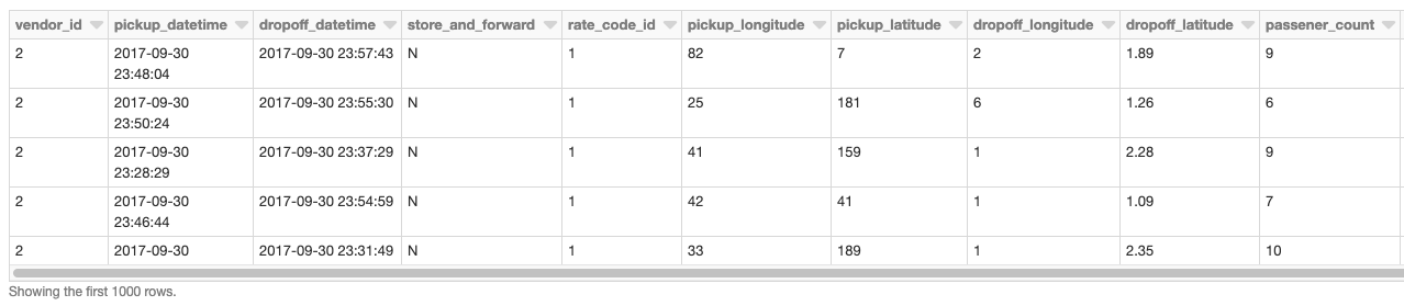
The examples which follow are generally oriented around a NYC taxi pickup / dropoff dataset found here. NYC Taxi Zone data with geometries will also be used as the set of polygons. This data contains polygons for the five boroughs of NYC as well the neighborhoods. This notebook will walk you through preparations and cleanings done to convert the initial CSV files into Delta Lake Tables as a reliable and performant data source.

Our base DataFrame is the taxi pickup / dropoff data read from a Delta Lake Table using Databricks.

%scala
val dfRaw = spark.read.format("delta").load("/ml/blogs/geospatial/delta/nyc-green") 
display(dfRaw) // showing first 10 columns

Example geospatial data read from a Delta Lake table using Databricks.

Geospatial Operations using GeoSpatial Libraries for Apache Spark

Over the last few years, several libraries have been developed to extend the capabilities of Apache Spark for geospatial analysis. These frameworks bear the brunt of registering commonly applied user defined types (UDT) and functions (UDF) in a consistent manner, lifting the burden otherwise placed on users and teams to write ad-hoc spatial logic. Please note that in this blog post we use several different spatial frameworks chosen to highlight various capabilities. We understand that other frameworks exist beyond those highlighted which you might also want to use with Databricks to process your spatial workloads.

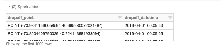
Earlier, we loaded our base data into a DataFrame. Now we need to turn the latitude/longitude attributes into point geometries. To accomplish this, we will use UDFs to perform operations on DataFrames in a distributed fashion. Please refer to the provided notebooks at the end of the blog for details on adding these frameworks to a cluster and the initialization calls to register UDFs and UDTs. For starters, we have added GeoMesa to our cluster, a framework especially adept at handling vector data. For ingestion, we are mainly leveraging its integration of JTS with Spark SQL which allows us to easily convert to and use registered JTS geometry classes. We will be using the function st_makePoint that given a latitude and longitude create a Point geometry object. Since the function is a UDF, we can apply it to columns directly.

%scala
val df = dfRaw
 .withColumn("pickup_point", st_makePoint(col("pickup_longitude"), col("pickup_latitude")))
 .withColumn("dropoff_point", st_makePoint(col("dropoff_longitude"),col("dropoff_latitude")))
display(df.select("dropoff_point","dropoff_datetime"))

Using UDFs to perform operations on DataFrames in a distributed fashion to turn geospatial data latitude/longitude attributes into point geometries.

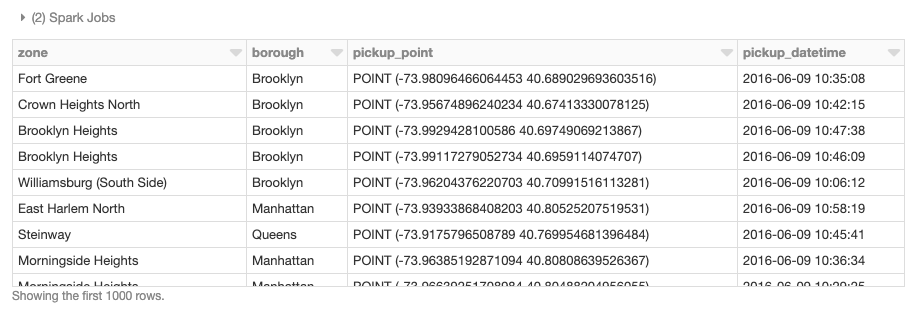
We can also perform distributed spatial joins, in this case using GeoMesa’s provided st_contains UDF to produce the resulting join of all polygons against pickup points.

%scala
val joinedDF = wktDF.join(df, st_contains($"the_geom", $"pickup_point")
display(joinedDF.select("zone","borough","pickup_point","pickup_datetime"))

Using GeoMesa’s provided st_contains UDF, for example, to produce the resulting join of all polygons against pickup points.

Wrapping Single-node Libraries in UDFs

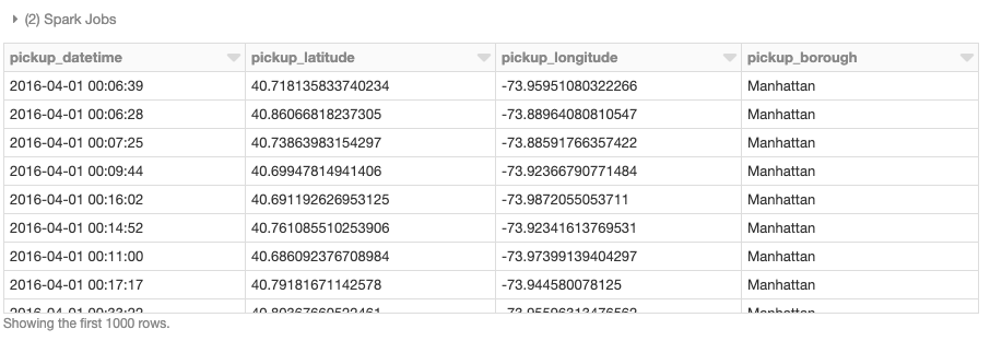
In addition to using purpose built distributed spatial frameworks, existing single-node libraries can also be wrapped in ad-hoc UDFs for performing geospatial operations on DataFrames in a distributed fashion. This pattern is available to all Spark language bindings – Scala, Java, Python, R, and SQL – and is a simple approach for leveraging existing workloads with minimal code changes. To demonstrate a single-node example, let’s load NYC borough data and define UDF find_borough(…) for point-in-polygon operation to assign each GPS location to a borough using geopandas. This could also have been accomplished with a vectorized UDF for even better performance.

%python 
# read the boroughs polygons with geopandas
gdf = gdp.read_file("/dbfs/ml/blogs/geospatial/nyc_boroughs.geojson")

b_gdf = sc.broadcast(gdf) # broadcast the geopandas dataframe to all nodes of the cluster 
def find_borough(latitude,longitude):
  mgdf = b_gdf.value.apply(lambda x: x["boro_name"] if x["geometry"].intersects(Point(longitude, latitude))
  idx = mgdf.first_valid_index()
  return mgdf.loc[idx] if idx is not None else None

find_borough_udf = udf(find_borough, StringType())

Now we can apply the UDF to add a column to our Spark DataFrame which assigns a borough name to each pickup point.

%python 
# read the coordinates from delta 
df = spark.read.format("delta").load("/ml/blogs/geospatial/delta/nyc-green")
df_with_boroughs = df.withColumn("pickup_borough", find_borough_udf(col("pickup_latitude"),col(pickup_longitude)))
display(df_with_boroughs.select(
  "pickup_datetime","pickup_latitude","pickup_longitude","pickup_borough"))

The result of a single-node example, where Geopandas is used to assign each GPS location to NYC borough.

Grid Systems for Spatial Indexing

Geospatial operations are inherently computationally expensive. Point-in-polygon, spatial joins, nearest neighbor or snapping to routes all involve complex operations. By indexing with grid systems, the aim is to avoid geospatial operations altogether. This approach leads to the most scalable implementations with the caveat of approximate operations. Here is a brief example with H3.

Scaling spatial operations with H3 is essentially a two step process. The first step is to compute an H3 index for each feature (points, polygons, …) defined as UDF geoToH3(…). The second step is to use these indices for spatial operations such as spatial join (point in polygon, k-nearest neighbors, etc), in this case defined as UDF multiPolygonToH3(…).

%scala 
import com.uber.h3core.H3Core
import com.uber.h3core.util.GeoCoord
import scala.collection.JavaConversions._
import scala.collection.JavaConverters._

object H3 extends Serializable {
  val instance = H3Core.newInstance()
}

val geoToH3 = udf{ (latitude: Double, longitude: Double, resolution: Int) => 
  H3.instance.geoToH3(latitude, longitude, resolution) 
}
                  
val polygonToH3 = udf{ (geometry: Geometry, resolution: Int) => 
  var points: List[GeoCoord] = List()
  var holes: List[java.util.List[GeoCoord]] = List()
  if (geometry.getGeometryType == "Polygon") {
    points = List(
      geometry
        .getCoordinates()
        .toList
        .map(coord => new GeoCoord(coord.y, coord.x)): _*)
  }
  H3.instance.polyfill(points, holes.asJava, resolution).toList 
}

val multiPolygonToH3 = udf{ (geometry: Geometry, resolution: Int) => 
  var points: List[GeoCoord] = List()
  var holes: List[java.util.List[GeoCoord]] = List()
  if (geometry.getGeometryType == "MultiPolygon") {
    val numGeometries = geometry.getNumGeometries()
    if (numGeometries > 0) {
      points = List(
        geometry
          .getGeometryN(0)
          .getCoordinates()
          .toList
          .map(coord => new GeoCoord(coord.y, coord.x)): _*)
    }
    if (numGeometries > 1) {
      holes = (1 to (numGeometries - 1)).toList.map(n => {
        List(
          geometry
            .getGeometryN(n)
            .getCoordinates()
            .toList
            .map(coord => new GeoCoord(coord.y, coord.x)): _*).asJava
      })
    }
  }
  H3.instance.polyfill(points, holes.asJava, resolution).toList 
}

We can now apply these two UDFs to the NYC taxi data as well as the set of borough polygons to generate the H3 index.

%scala
val res = 7 //the resolution of the H3 index, 1.2km
val dfH3 = df.withColumn(
  "h3index",
  geoToH3(col("pickup_latitude"), col("pickup_longitude"), lit(res))
)
val wktDFH3 = wktDF
  .withColumn("h3index", multiPolygonToH3(col("the_geom"), lit(res)))
  .withColumn("h3index", explode($"h3index"))

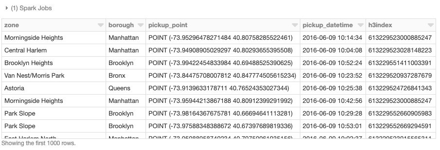
Given a set of a lat/lon points and a set of polygon geometries, it is now possible to perform the spatial join using h3index field as the join condition. These assignments can be used to aggregate the number of points that fall within each polygon for instance. There are usually millions or billions of points that have to be matched to thousands or millions of polygons which necessitates a scalable approach. There are other techniques not covered in this blog which can be used for indexing in support of spatial operations when an approximation is insufficient.

%scala
val dfWithBoroughH3 = dfH3.join(wktDFH3,"h3index") 
    
display(df_with_borough_h3.select("zone","borough","pickup_point","pickup_datetime","h3index"))

DataFrame table representing the spatial join of a set of lat/lon points and polygon geometries, using a specific field as the join condition.

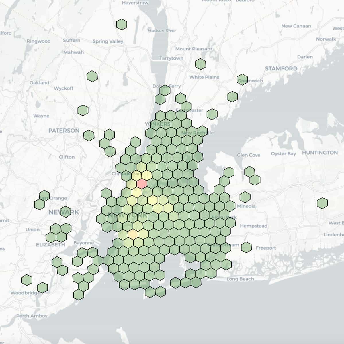
Here is a visualization of taxi dropoff locations, with latitude and longitude binned at a resolution of 7 (1.22km edge length) and colored by aggregated counts within each bin.

Geospatial visualization of taxi dropoff locations, with latitude and longitude binned at a resolution of 7 (1.22km edge length) and colored by aggregated counts within each bin.

Handling Spatial Formats with Databricks

Geospatial data involves reference points, such as latitude and longitude, to physical locations or extents on the earth along with features described by attributes. While there are many file formats to choose from, we have picked out a handful of representative vector and raster formats to demonstrate reading with Databricks.

Vector Data

Vector data is a representation of the world stored in x (longitude), y (latitude) coordinates in degrees, also z (altitude in meters) if elevation is considered. The three basic symbol types for vector data are points, lines, and polygons. Well-known-text (WKT), GeoJSON, and Shapefile are some popular formats for storing vector data we highlight below.

Let’s read NYC Taxi Zone data with geometries stored as WKT. The data structure we want to get back is a DataFrame which will allow us to standardize with other APIs and available data sources, such as those used elsewhere in the blog. We are able to easily convert the WKT text content found in field the_geom into its corresponding JTS Geometry class through the st_geomFromWKT(…) UDF call.

%scala
val wktDFText = sqlContext.read.format("csv")
 .option("header", "true")
 .option("inferSchema", "true")
 .load("/ml/blogs/geospatial/nyc_taxi_zones.wkt.csv")

val wktDF = wktDFText.withColumn("the_geom", st_geomFromWKT(col("the_geom"))).cache

GeoJSON is used by many open source GIS packages for encoding a variety of geographic data structures, including their features, properties, and spatial extents. For this example, we will read NYC Borough Boundaries with the approach taken depending on the workflow. Since the data is conforming JSON, we could use the Databricks built-in JSON reader with .option(“multiline”,”true”) to load the data with the nested schema.

%python
json_df = spark.read.option("multiline","true").json("nyc_boroughs.geojson")

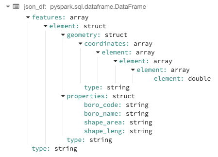
Example of using the Databricks built-in JSON reader .option(“multiline”,”true”) to load the data with the nested schema.

From there we could choose to hoist any of the fields up to top level columns using Spark’s built-in explode function. For example, we might want to bring up geometry, properties, and type and then convert geometry to its corresponding JTS class as was shown with the WKT example.

%python
from pyspark.sql import functions as F
json_explode_df = ( json_df.select(
 "features",
 "type",
 F.explode(F.col("features.properties")).alias("properties")
).select("*",F.explode(F.col("features.geometry")).alias("geometry")).drop("features"))

display(json_explode_df)

Using the Spark’s built-in explode function to raise a field to the top level, displayed within a DataFrame table.

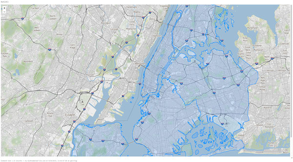
We can also visualize the NYC Taxi Zone data within a notebook using an existing DataFrame or directly rendering the data with a library such as Folium, a Python library for rendering spatial data. Databricks File System (DBFS) runs over a distributed storage layer which allows code to work with data formats using familiar file system standards. DBFS has a FUSE Mount to allow local API calls which perform file read and write operations,which makes it very easy to load data with non-distributed APIs for interactive rendering. In the Python open(…) command below, the “/dbfs/…” prefix enables the use of FUSE Mount.

%python 
import folium
import json

with open ("/dbfs/ml/blogs/geospatial/nyc_boroughs.geojson", "r") as myfile:
 boro_data=myfile.read() # read GeoJSON from DBFS using FuseMount

m = folium.Map(
 location=[40.7128, -74.0060],
 tiles='Stamen Terrain',
 zoom_start=12 
)
folium.GeoJson(json.loads(boro_data)).add_to(m)
m # to display, also could use displayHTML(...) variants

We can also visualize the NYC Taxi Zone data, for example, within a notebook using an existing DataFrame or directly rendering the data with a library such as Folium, a Python library for rendering geospatial data.

Shapefile is a popular vector format developed by ESRI which stores the geometric location and attribute information of geographic features. The format consists of a collection of files with a common filename prefix (*.shp, *.shx, and *.dbf are mandatory) stored in the same directory. An alternative to shapefile is KML, also used by our customers but not shown for brevity. For this example, let’s use NYC Building shapefiles. While there are many ways to demonstrate reading shapefiles, we will give an example using GeoSpark. The built-in ShapefileReader is used to generate the rawSpatialDf DataFrame.

%scala
var spatialRDD = new SpatialRDD[Geometry]
spatialRDD = ShapefileReader.readToGeometryRDD(sc, "/ml/blogs/geospatial/shapefiles/nyc")

var rawSpatialDf = Adapter.toDf(spatialRDD,spark)
rawSpatialDf.createOrReplaceTempView("rawSpatialDf") //DataFrame now available to SQL, Python, and R 

By registering rawSpatialDf as a temp view, we can easily drop into pure Spark SQL syntax to work with the DataFrame, to include applying a UDF to convert the shapefile WKT into Geometry.

%sql 
SELECT *,
 ST_GeomFromWKT(geometry) AS geometry -- GeoSpark UDF to convert WKT to Geometry 
FROM rawspatialdf 

Additionally, we can use Databricks built in visualization for inline analytics such as charting the tallest buildings in NYC.

%sql 
SELECT name, 
 round(Cast(num_floors AS DOUBLE), 0) AS num_floors --String to Number
FROM rawspatialdf 
WHERE name <> ''
ORDER BY num_floors DESC LIMIT 5

A Databricks built-in visualization for inline analytics charting, for example, the tallest buildings in NYC.

Raster Data

Raster data stores information of features in a matrix of cells (or pixels) organized into rows and columns (either discrete or continuous). Satellite images, photogrammetry, and scanned maps are all types of raster-based Earth Observation (EO) data.

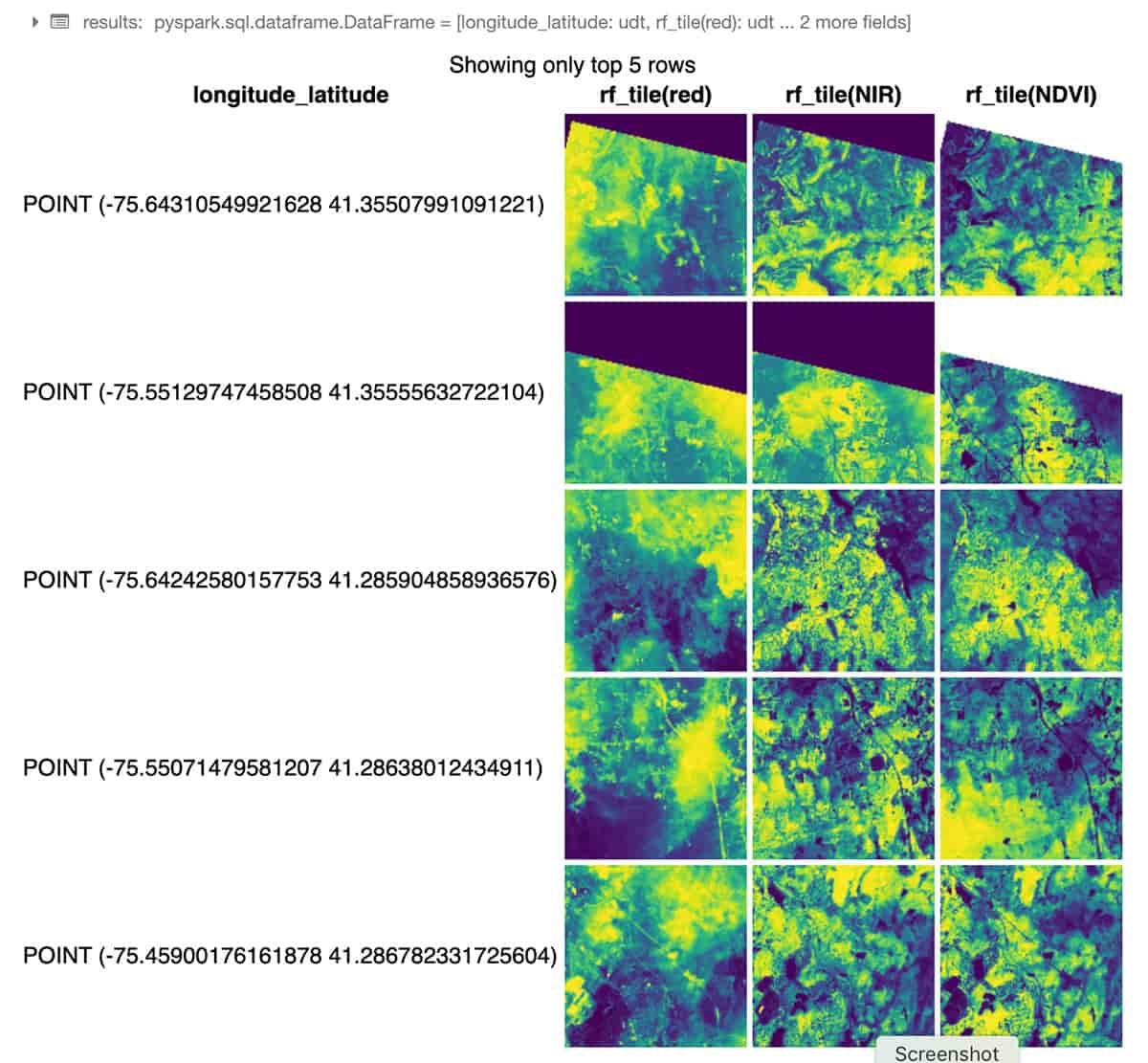
The following Python example uses RasterFrames, a DataFrame-centric spatial analytics framework, to read two bands of JPEG2000 Landsat-8 imagery (red and near-infrared) and combine them into Normalized Difference Vegetation Index. We can use this data to assess plant health around NYC. The rf_ipython module is used to manipulate RasterFrame contents into a variety of visually useful forms, such as below where the red, NIR and NDVI tile columns are rendered with color ramps, using the Databricks built-in displayHTML(…) command to show the results within the notebook.

%python
# construct a CSV "catalog" for RasterFrames `raster` reader 
# catalogs can also be Spark or Pandas DataFrames
bands = [f'B{b}' for b in [4, 5]]
uris = [f'https://landsat-pds.s3.us-west-2.amazonaws.com/c1/L8/014/032/LC08_L1TP_014032_20190720_20190731_01_T1/LC08_L1TP_014032_20190720_20190731_01_T1_{b}.TIF' for b in bands]
catalog = ','.join(bands) + '\n' + ','.join(uris)

# read red and NIR bands from Landsat 8 dataset over NYC
rf = spark.read.raster(catalog, bands) \
 .withColumnRenamed('B4', 'red').withColumnRenamed('B5', 'NIR') \
 .withColumn('longitude_latitude', st_reproject(st_centroid(rf_geometry('red')), rf_crs('red'), lit('EPSG:4326'))) \
 .withColumn('NDVI', rf_normalized_difference('NIR', 'red')) \
 .where(rf_tile_sum('NDVI') > 10000)

results = rf.select('longitude_latitude', rf_tile('red'), rf_tile('NIR'), rf_tile('NDVI'))
displayHTML(rf_ipython.spark_df_to_html(results))

RasterFrame contents can be filtered, transformed, summarized, resampled, and rasterized through 200+ raster and vector functions.

Through its custom Spark DataSource, RasterFrames can read various raster formats, including GeoTIFF, JP2000, MRF, and HDF, from an array of services. It also supports reading the vector formats GeoJSON and WKT/WKB. RasterFrame contents can be filtered, transformed, summarized, resampled, and rasterized through 200+ raster and vector functions, such as st_reproject(…) and st_centroid(…) used in the example above. It provides APIs for Python, SQL, and Scala as well as interoperability with Spark ML.

GeoDatabases

Geo databases can be filebased for smaller scale data or accessible via JDBC / ODBC connections for medium scale data. You can use Databricks to query many SQL databases with the built-in JDBC / ODBC Data Source. Connecting to PostgreSQL is shown below which is commonly used for smaller scale workloads by applying PostGIS extensions. This pattern of connectivity allows customers to maintain as-is access to existing databases.

%scala
display(
  sqlContext.read.format("jdbc")
    .option("url", jdbcUrl)
    .option("driver", "org.postgresql.Driver")
    .option("dbtable", 
      """(SELECT * FROM yellow_tripdata_staging 
      OFFSET 5 LIMIT 10) AS t""") //predicate pushdown
    .option("user", jdbcUsername)
    .option("jdbcPassword", jdbcPassword)
  .load)

Getting Started with Geospatial Analysis on Databricks

Businesses and government agencies seek to use spatially referenced data in conjunction with enterprise data sources to draw actionable insights and deliver on a broad range of innovative use cases. In this blog we demonstrated how the Databricks Unified Data Analytics Platform can easily scale geospatial workloads, enabling our customers to harness the power of the cloud to capture, store and analyze data of massive size.

In an upcoming blog, we will take a deep dive into more advanced topics for geospatial processing at-scale with Databricks. You will find additional details about the spatial formats and highlighted frameworks by reviewing Data Prep Notebook, GeoMesa + H3 Notebook, GeoSpark Notebook, GeoPandas Notebook, and Rasterframes Notebook. Also, stay tuned for a new section in our documentation specifically for geospatial topics of interest.

--

Try Databricks for free. Get started today.

The post Processing Geospatial Data at Scale With Databricks appeared first on Databricks.

Streamlining Variant Normalization on Large Genomic Datasets with Glow

Cross posted from the Glow blog.

Many research and drug development projects in the genomics world involve large genomic variant data sets, the volume of which has been growing exponentially over the past decade. However, the tools to extract, transform, load (ETL) and analyze these data sets have not kept pace with this growth. Single-node command line tools or scripts are very inefficient in handling terabytes of genomics data in these projects. In October of this year, Databricks and the Regeneron Genetics Center partnered to introduce project Glow, an open-source toolkit for large-scale genomic analysis based on Apache Spark™, to address this issue. An optimized version of Glow is incorporated into Databricks Unified Data Analytics Platform (UDAP) for Genomics, which in addition to several feature optimizations, provides many more secondary and tertiary analysis features on top of a scalable, managed cloud service, making Databricks the best platform to run Glow.

In large cross-team research or drug discovery projects, computational biologists and bioinformaticians usually need to merge very large variant call sets in order to perform downstream analyses. In a prior post, we showcased the power and simplicity of Glow in ETL and merging of variant call sets from different sources using Glow’s VCF and BGEN Data Sources at unprecedented scales. Differently sourced variant call sets impose another major challenge. It is not uncommon for these sets to be generated by different variant calling tools and methods. Consequently, the same genomic variant may be represented differently (in terms of genomic position and alleles) across different call sets. These discrepancies in variant representation must be resolved before any further analysis on the data. This is critical for the following reasons:

1. To avoid incorrect bias in the results of downstream analysis on the merged set of variants or waste of analysis effort on seemingly new variants due to lack of normalization, which are in fact redundant (see Tan et al. for examples of this redundancy in 1000 Genome Project variant calls and dbSNP)
2. To ensure that the merged data set and its post-analysis derivations are compatible and comparable with other public and private variant databases.

This is achieved by what is referred to as variant normalization, a process that ensures the same variant is represented identically across different data sets. Performing variant normalization on terabytes of variant data in large projects using popular single-node tools can become quite a challenge as the acceptable input and output of these tools are the flat file formats that are commonly used to store variant calls (such as VCF and BGEN). To address this issue, we introduced the variant normalization transformation into Glow, which directly acts on a Spark Dataframe of variants to generate a DataFrame of normalized variants, harnessing the power of Spark to normalize variants from hundreds of thousands of samples in a fast and scalable manner with just a single line of Python or Scala code. Before addressing our normalizer, let us have a slightly more technical look at what variant normalization actually does.

What does variant normalization do?

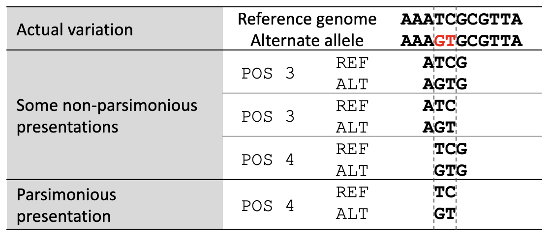
Variant normalization ensures that the representation of a variant is both “parsimonious” and “left-aligned.” A variant is parsimonious if it is represented in as few nucleotides as possible without reducing the length of any allele to zero. An example is given in Figure 1.

Figure 1. Variant Parsimony

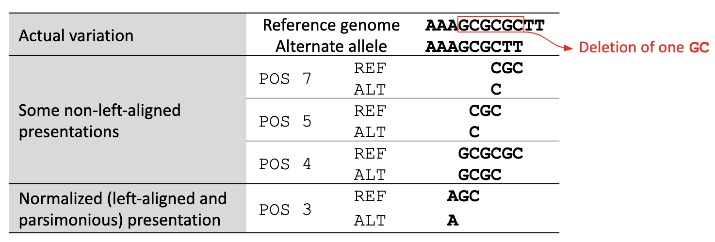
A variant is left-aligned if its position cannot be shifted to the left while keeping the length of all its alleles the same. An example is given in Figure 2.

Figure 2. Left-aligned Variant

Tan et al. have proved that normalization results in uniqueness. In other words, two variants have different normalized representations if and only if they are actually different variants.

Variant normalization in Glow

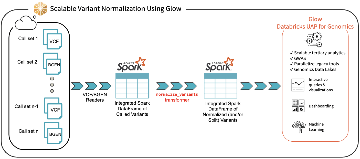
We have introduced the normalize_variants transformer into Glow (Figure 3). After ingesting variant calls into a Spark DataFrame using the VCF, BGEN or Delta readers, a user can call a single line of Python or Scala code to normalize all variants. This generates another DataFrame in which all variants are presented in their normalized form. The normalized DataFrame can then be used for downstream analyses like a GWAS using our built-in regression functions or an efficiently-parallelized GWAS tool.

Figure 3. Scalable Variant Normalization Using Glow

The normalize_variants transformer brings unprecedented scalability and simplicity to this important upstream process, hence is yet another reason why Glow and Databricks UDAP for Genomics are ideal platforms for biobank-scale genomic analyses, e.g., association studies between genetic variations and diseases across cohorts of hundreds of thousands of individuals.

The underlying normalization algorithm and its accuracy

There are several single-node tools for variant normalization that use different normalization algorithms. Widely used tools for variant normalization include vt normalize, bcftools norm, and the GATK’s LeftAlignAndTrimVariants.

Based on our own investigation and also as indicated by Bayat et al. and Tan et al., the GATK’s LeftAlignAndTrimVariants algorithm frequently fails to completely left-align some variants. For example, we noticed that on the test_left_align_hg38.vcf test file from GATK itself, applying LeftAlignAndTrimVariants results in an incorrect normalization of 3 of the 16 variants in the file, including the variants at positions chr20:63669973, chr20:64012187, and chr21:13255301. These variants are normalized correctly using vt normalize and bcftools norm.

Consequently, in our normalize_variants transformer, we used an improved version of the bcftools norm or vt normalize algorithms, which are similar in fundamentals. For a given variant, we start by right-trimming all the alleles of the variant as long as their rightmost nucleotides are the same. If the length of any allele reaches zero, we left-append it with a fixed block of nucleotides from the reference genome (the nucleotides are added in blocks as opposed to one-by-one to limit the number of referrals to the reference genome). When right-trimming is terminated, a potential left-trimming is performed to eliminate the leftmost nucleotides common to all alleles (possibly generated by prior left-appendings). The start, end, and alleles of the variants are updated appropriately during this process.

We benchmarked the accuracy of our normalization algorithm against vt normalize and bcftools norm on multiple test files and validated that our results match the results of these tools.

The optional splitting of multiallelic variants

Our normalize_variants transformer can optionally split multiallelic variants to biallelics. This is controlled by the mode option that can be supplied to this transformer. The possible values for the mode option are as follows: normalize (default), which performs normalization only, split_and_normalize, which splits multiallelic variants to biallelic ones before performing normalization, and split, which only splits multiallelics without doing any normalization.

The splitting logic of our transformer is the same as the splitting logic followed by GATK’s LeftAlignAndTrimVariants tool using –splitMultiallelics option. More precisely, in case of splitting multiallelic variants loaded from VCF files, this transformer recalculates the GT blocks for the resulting biallelic variants if possible, and drops all INFO fields, except for AC, AN, and AF. These three fields are imputed based on the newly calculated GT blocks, if any exists, otherwise, these fields are dropped as well.

Using the normalize_variant transformer

Here, we briefly demonstrate how using Glow very large variant call sets can be normalized and/or split. First, VCF and/or BGEN files can be read into a Spark DataFrame as demonstrated in a prior post. This is shown in Python for the set of VCF files contained in a folder named /databricks-datasets/genomics/call-sets:

original_variants_df = spark.read\
  .format("vcf")\
  .option("includeSampleIds", False)\
  .load("/databricks-datasets/genomics/call-sets")

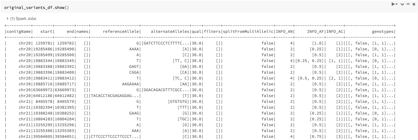
An example of the DataFrame original_variants_df is shown in Figure 4.

Figure 4. The variant DataFrame original_variants_df

The variants can then be normalized using the normalize_variants transformer as follows:

import glow

ref_genome_path = '/mnt/dbnucleus/dbgenomics/grch38/data/GRCh38.fa'

normalized_variants_df = glow.transform(\
  "normalize_variants",\
  original_variants_df,\
  reference_genome_path=ref_genome_path\
)

Note that normalization requires the reference genome .fasta or .fa file, which is provided using the reference_genome_path option. The .dict and .fai files must accompany the reference genome file in the same folder (read more about these file formats here).

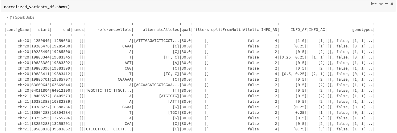
Our example Dataframe after normalization can be seen in Figure 5.

Figure 5. The normalized_variants_df DataFrame obtained after applying normalize_variants transformer on original_variants_df. Notice that several variants are normalized and their start, end, and alleles have changed accordingly.

By default, the transformer normalizes each variant without splitting the multiallelic variants before normalization as seen in Figure 5. By setting the mode option to split_and_normalize, nothing changes for biallelic variants, but the multiallelic variants are first split to the appropriate number of biallelics and the resulting biallelics are normalized. This can be done as follows:

split_and_normalized_variants_df = glow.transform(\
  "normalize_variants",\
  original_variants_df,\
  reference_genome_path=ref_genome_path,\
  mode=“split_and_normalize”
)

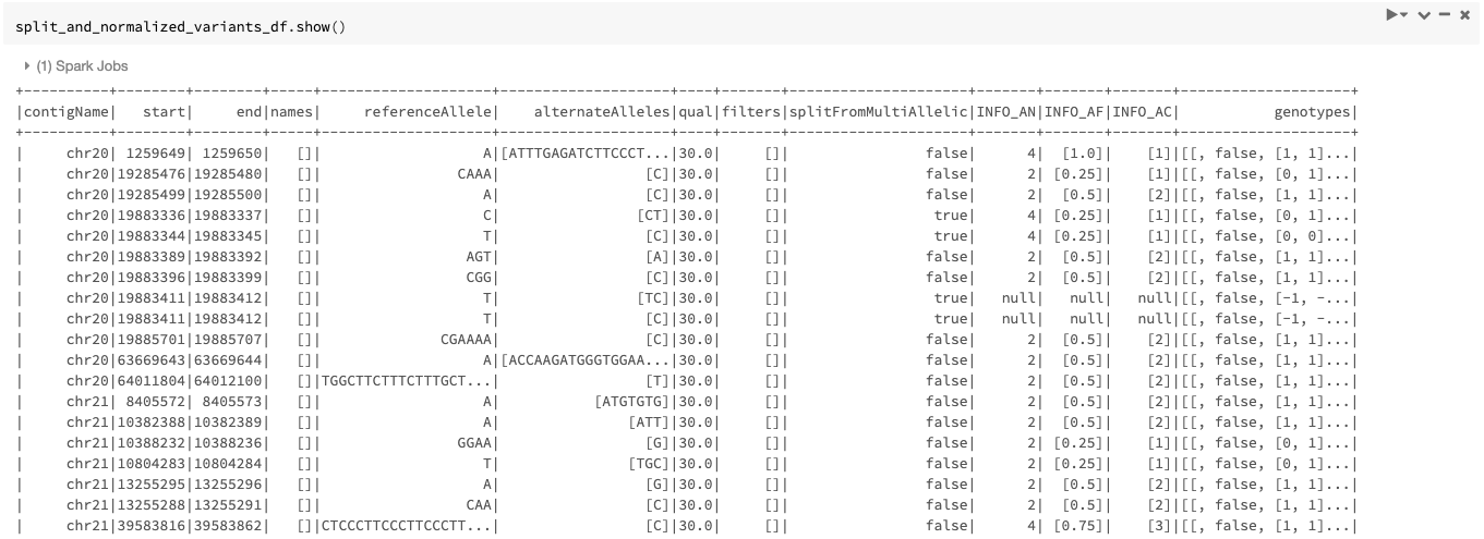
The resulting DataFrame looks like Figure 6.

Figure 6. The split_and_normalized_variants_df DataFrame after applying normalize_variants transformer with mode=“split_and_normalize” on original_variants_df. Notice that for example the triallelic variant (chr20, start=19883344, end=19883345, REF=T, ALT=[TT,C]) of original_variants_df has been split into two biallelic variants and then normalized resulting in two normalized biallelic variants (chr20, start=19883336, end=19883337, REF=C, ALT=CT) and (chr20, start=19883344, end=19883345, REF=T, ALT=C).

As mentioned before, the transformer can also be used only for splitting of multiallelics without doing any normalization by setting the mode option to split.

Summary

Using Glow normalize_variants transformer, computational biologists and bioinformaticians can normalize very large variant datasets of hundreds of thousands of samples in a fast and scalable manner. Differently sourced call sets can be ingested and merged using VCF and/or BGEN readers, normalization can be performed using this transformer in a just a single line of code. The transformer can optionally perform splitting of multiallelic variants to biallelics as well.

Get started with Glow — Streamline variant normalization

Our normalize_variants transformer makes it easy to normalize (and split) large variant datasets with a very small amount of code (Azure | AWS). Learn more about Glow features here and check out Databricks Unified Data Analytics for Genomics or try out a preview today.

 

References

Arash Bayat, Bruno Gaëta, Aleksandar Ignjatovic, Sri Parameswaran, Improved VCF normalization for accurate VCF comparison, Bioinformatics, Volume 33, Issue 7, 2017, Pages 964–970

Adrian Tan, Gonçalo R. Abecasis, Hyun Min Kang, Unified representation of genetic variants, Bioinformatics, Volume 31, Issue 13, 2015, Pages 2202–2204

Additional Resources

• Docs > Glow
• Scaling Genomic Workflows with Spark SQL BGEN and VCF Readers
• Engineering population scale Genome-Wide Association Studies with Apache Spark™, Delta Lake, and MLflow
• Parallelizing SAIGE Across Hundreds of Cores

--

Try Databricks for free. Get started today.

The post Streamlining Variant Normalization on Large Genomic Datasets with Glow appeared first on Databricks.

Big Data is Transforming the Financial Industry at its Core

Earlier this year, Investopedia published a very insightful article on the intersection of big data and the financial industry. Big data is changing every facet of the financial industry, from insurance actuary processes to the management of the stock market.

The Progression of Big Data Technology in the Financial Industry

The 21st has been the age of information technology. Information technology and the accumulation of truly staggering amounts of data have transformed the landscapes of countless industries, signaling a paradigm shift in the way we do things.

One of the most acutely affected industries has been the financial industry. This industry thrives on processing market information to figure out what the next big thing is and what to do about it. With the rise of big data, the financial industry has undergone a metamorphosis on a scale rarely seen in nature.

MAPR cited some hard statistics on the role of big data in the financial services industry. They showed that the global big data market is worth $130.1 billion. The demand for big data in the financial services industry accounts for 13.1% of this market – or $17 billion. Other financial sectors are also utilizing big data and presumably account for around 20% or ...


Read More on Datafloq

IITs eye Asean footprint to boost global ranking

The presence of few international students on their campuses has been a major hindrance in stepping up their game in global rankings.

Made in India, Made for the World

After Pichai took over, there have been around 20 India-specific initiatives, some of them for global markets, but always first tested and launched in India.

Diversity and Cybersecurity: How can Diverse Security Teams Empower Organizations?

In most cybersecurity conversations, most people tend to overlook the pressing issue of diversity in the cybersecurity industry as a whole. Not only is the cybersecurity world made up of a highly homogenous group of people at the top, the lack of diversity actually creates hurdles and makes the process of securing an enterprise harder than it has to be. 

Usually, workplace diversity is looked at as a buzzing ‘fad’ and is unfortunately seen by enterprise owners as a means to project a certain image, rather than being something that they are genuinely passionate about. 

However, as far as the cybersecurity world is concerned, making diversity mainstream is far more critical than previously thought. Unlike other avenues where the issue of workplace diversity is usually seen through the perspective of moral or ethical debate- having a diverse security team can actually equip enterprises better against external and internal threats. 

As more and more businesses ride the wave of digitalization, which relies on the inclusion of faulty technologies such as cloud computing within an enterprise- the surface area available to cybercriminals expands, which ultimately leads to hackers attacking with an extremely wide range of tools at their disposal.

 As the threats faced by enterprises continue ...


Read More on Datafloq

Databricks and Informatica Integration Simplifies Data Lineage and Governance for Cloud Analytics

In a rapidly evolving world of big data, data discovery, governance and data lineage is an essential aspect of data management. As organizations modernize their workloads into multi-cloud and hybrid environments, data starts to get distributed across cloud data lakes and SaaS applications. With that, organizations are trying to answer key questions:

• How do I find the right dataset?
• How do I ensure the data is of high quality?
• How do I move faster to deliver insights for analytics and ML workloads?
• How do I comply with regulations and deliver trusted data?

Achieving data discovery, lineage and reliability – at enterprise scale – is an opportunity for organizations. To help enterprises build a strong foundation for data management, we’ve partnered with Informatica to provide an end-to-end lineage solution. This joint solution provides complete visibility and traceability into data pipelines on Delta Lake, the open-source storage layer for reliable data lakes at scale.

Building End-to-End Pipelines with Data Discovery, Governance and Lineage in the Cloud on Delta Lake

Take a moment to think about all the applications we use everyday – email, web, mobile, social media, SaaS applications, BI, reporting dashboards and many others. Data Engineers spend vast amounts of time in these applications finding datasets and tracing data transformations, which delays analytics and machine learning projects.

The joint solution by Databricks and Informatica solves this problem by enabling data engineers and data scientists to find, validate and trace datasets as they move through data pipelines. Informatica’s EDC connects seamlessly with Delta Lake to scan and index metadata so teams can discover and profile data and find detailed lineage of that data as it moves through pipelines. This allows data engineers and data scientists to easily track data movement, including column/metric-level lineage to identify related tables, views and domains.

Along with EDC, Databricks integrates with Informatica Data Engineering Integration (DEI). DEI uses dynamic mappings and data transformations to ingest data from multiple source systems and applications into Delta tables with complete data lineage tracking. Once the data is in Delta tables, EDC performs scanning, profiling and discovery to help data engineers find the right data sets.

Viewing Lineage of Delta Datasets Engineered with Informatica Data Engineering Integration in EDC

Data Governance at Enterprise Scale

With new and upcoming regulations such as the General Data Protection Regulation (GDPR) and California Consumer Privacy Act (CCPA), data governance becomes integral to any data management initiative. For example, GDPR mandates ‘Right to Access’ that allows a customer to view their personal information across the entire enterprise. Similarly, the Right to Erasure requires that all their personal data be deleted without delay. Since Delta is a transactional engine, specific data (i.e. rows in tables) can be easily deleted using DELETE commands in the ‘Right to be forgotten’ compliance scenarios, without the burden of coding elaborate pipelines.

Overall, with data dispersed across disparate sources, it can be challenging to keep track of what data resides where and which on-premise and cloud workflows touch that data. A cloud-based data platform and discovery program for the entire organization can future proof its data governance discipline.

Getting started with the Databricks-Informatica End-to-end Data Lineage solution

Building intelligent data pipelines to bring data from different silos, tracing its origin and creating a complete view of data movement in the cloud is critical to enterprise organizations. The Databricks and Informatica partnership enables modern data teams to leverage data assets to scale and document datasets and data pipelines for analytics and ML. It is a powerful integration for data engineers and data scientists looking to automate their governance processes while achieving speed and agility of data management for the future.

Check out this webinar for an in-depth demo of the Databricks and Informatica joint solution for data lineage.
https://pages.databricks.com/201911-WB-Data-Discovery-Lineage-Analytics-DB-Informatica_03.On-demandpage.html

Related Resources

• Databricks and Informatica Accelerate Development and Complete Data Governance for Intelligent Data Pipelines
• Delta Lake – Brings data reliability and performance to your data lakes
• Enterprise Data Governance and Compliance at Scale

--

Try Databricks for free. Get started today.

The post Databricks and Informatica Integration Simplifies Data Lineage and Governance for Cloud Analytics appeared first on Databricks.

Ten Trends of IoT in 2020

The Internet of Things (IoT) is actively shaping both the industrial and consumer worlds. Smart tech finds its way to every business and consumer domain there is — from retail to healthcare, from finances to logistics — and a missed opportunity strategically employed by a competitor can easily qualify as a long-term failure for companies who don’t innovate [3]. The year 2020 will hit all 4 components of IoT Model: Sensors, Networks (Communications), Analytics (Cloud), and Applications, with different degrees of impact.

By 2020, the Internet of Things (IoT) is predicted to generate an additional $344B in revenues, as well as to drive $177B in cost reductions. IoT and smart devices are already increasing the performance metrics of major US-based factories. They are in the hands of employees, covering routine management issues and boosting their productivity by 40–60% [1]. The following 10 trends explore the impact of many technologies on IoT and predict what is next for IoT (see Figure 1).



Figure 1: 10 Trends of IoT in 2020.

IoT Prediction 1: Growth in Data and Devices with More Human-Device Interaction

By the end of 2019, there will be are around 3.6 billion devices that are actively connected to the Internet and used for ...


Read More on Datafloq

Google co-founders step aside as Pichai takes helm of parent Alphabet

Streamlining management could help Alphabet better respond to the challenges and focus on growing profits, investors said.

As AI tech proliferates, India should update its patent laws: CII-TCS report

Software is no longer limited to traditional rule-based systems and has increasingly turned heuristic, showing higher intelligence than rule-based systems, it said.

Vikram lander debris: The engineer who cracked it for India

A 33-year-old space science enthusiast searched NASA moon craft images days on end to spot the elusive Indian moon lander that crashed into its surface

Top AI Trends Every Data Scientists and Engineers Must Not Miss in 2020

As we’ve trodden the path of 2019 with much galore in AI and the big data realm, we look back on a year whose start already saw the AI revolution. But what does 2020 have in store for us?

You’ll be surprised to know that 2020 will be a crucial year for AI adoption.

The artificial intelligence market continues to rise at breakneck speed. As predicted by IDC, the global spending on AI systems is said to reach USD 97.9 billion in 2023. Simply put, the coming year will be critical to set foot for the next innovation to take place.

What follows is the top emerging trends every AI specialist, AI engineer, and data scientist must take heed:

Deployment to lower power gets easier in AI

AI that uses 32-bit floating-point math is available in high-computing systems as well as clusters, data centers, and GPUs. The purpose of this is to avail of relevant results and to have easy training of models. However, this ruled out the lower cost and low power devices that use fixed-point math.

Also, there have been recent advances in software tools that support AI interference models having different levels of fixed-point math. This advancement has helped the deployment of ...


Read More on Datafloq

I was hooked to NASA's moon surface images for days: Chennai techie who found lost Vikram Lander

In a post on its website early on Tuesday, NASA has said its moon mission has discovered the remains of India’s Vikram Lander and identified the debris spotted by Subramanian with an “S” on its image.