
Turntables and vinyl records have made quite the comeback in recent years—record sales are at a 25 year high.
Turntables and vinyl records have made quite the comeback in recent years—record sales are at a 25 year high.

Standing desks are great for keeping you moving and your posture straight.

In an age where a lot of users want to keep their smartphones for as long as possible, DIY mobile phone repair has been gaining steam, and Ama…
Sorting Lego bricks is such a painful endeavor that most of us don’t even bother.

If you spend a lot of time at your desk, it’s important to arrange your workspace to minimize strain on your body and maximize comfort. …

If you have the original Echo still kicking it in your home, it might be time for an upgrade.
Next week we’ll be celebrating Customer Experience Day! October 2nd marks the 6th annual CX Day, which “celebrates the professionals and companies that make great customer experiences happen. It’s an opportunity to recognize great customer work, discover professional development opportunities, and strengthen professional networks.” (CXDay.org) Hortonworks has seen tremendous growth other the years, since its […]
The post In Our Customer’s Words – Previewing CX Day 2018 appeared first on Hortonworks.

You’d like to get into the drone sensation, but you don’t want to break the bank to do it.

Today, Facebook announced the new Oculus Quest, a standalone VR headset that features the same six degrees of freedom as the higher-end Oculus…
This is a community blog from Yinan Li, a software engineer at Google, working in the Kubernetes Engine team. He is part of the group of companies that have contributed to Kubernetes support in the upcoming Apache Spark 2.4.
Since the Kubernetes cluster scheduler backend was initially introduced in Apache Spark 2.3, the community has been working on a few important new features that make Spark on Kubernetes more usable and ready for a broader spectrum of use cases. The upcoming Apache Spark 2.4 release comes with a number of new features, some of which are highlighted below:
Below we will take a deeper look into each of the new features.
Soon to be released Spark 2.4 now supports running PySpark applications on Kubernetes. Both Python 2.x and 3.x are supported, and the major version of Python can be specified using the new configuration property spark.kubernetes.pyspark.pythonVersion, which can have value 2 or 3 but defaults to 2. Spark ships with a Dockerfile of a base image with the Python binding that is required to run PySpark applications on Kubernetes. Users can use the Dockerfile to build a base image or customize it to build a custom image.
Spark on Kubernetes now supports running R applications in the upcoming Spark 2.4. Spark ships with a Dockerfile of a base image with the R binding that is required to run R applications on Kubernetes. Users can use the Dockerfile to build a base image or customize it to build a custom image.
As one of the most requested features since the 2.3.0 release, client mode support is now available in the upcoming Spark 2.4. The client mode allows users to run interactive tools such as spark-shell or notebooks in a pod running in a Kubernetes cluster or on a client machine outside a cluster. Note that in both cases, users are responsible for properly setting up connectivity from the executors running in pods inside the cluster to the driver. When the driver runs in a pod in the cluster, the recommended way is to use a Kubernetes headless service to allow executors to connect to the driver using the FQDN of the driver pod. When the driver runs outside the cluster, however, it’s important for users to make sure that the driver is reachable from the executor pods in the cluster. For more detailed information on the client mode support, please refer to the documentation when Spark 2.4 is officially released.
In addition to the new features highlighted above, the Kubernetes cluster scheduler backend in the upcoming Spark 2.4 release has also received a number of bug fixes and improvements.
spark.kubernetes.executor.request.cores was introduced for configuring the physical CPU request for the executor pods in a way that conforms to the Kubernetes convention. For example, users can now use fraction values or millicpus like 0.5 or 500m. The value is used to set the CPU request for the container running the executor.The Spark driver running in a pod in a Kubernetes cluster no longer uses an init-container for downloading remote application dependencies, e.g., jars and files on remote HTTP servers, HDFS, AWS S3, or Google Cloud Storage. Instead, the driver uses spark-submit in client mode, which automatically fetches such remote dependencies in a Spark idiomatic way.
Users can now specify image pull secrets for pulling Spark images from private container registries, using the new configuration property spark.kubernetes.container.image.pullSecrets.
Users are now able to use Kubernetes secrets as environment variables through a secretKeyRef. This is achieved using the new configuration options spark.kubernetes.driver.secretKeyRef.[EnvName] and spark.kubernetes.executor.secretKeyRef.[EnvName] for the driver and executor, respectively.
The Kubernetes scheduler backend code running in the driver now manages executor pods using a level-triggered mechanism and is more robust to issues talking to the Kubernetes API server.
First of all, we would like to express huge thanks to Apache Spark and Kubernetes community contributors from multiple organizations (Bloomberg, Databricks, Google, Palantir, PepperData, Red Hat, Rockset and others) who have put tremendous efforts into this work and helped get Spark on Kubernetes this far. Looking forward, the community is working on or plans to work on features that further enhance the Kubernetes scheduler backend. Some of the features that are likely available in future Spark releases are listed below.
--
Try Databricks for free. Get started today.
The post What’s New for Apache Spark on Kubernetes in the Upcoming Apache Spark 2.4 Release appeared first on Databricks.

Having an organized bag can make or break your productivity levels—so why not spend more time getting w…

If you have a pair of hands, you may argue that you don’t need a shaving brush. And you know what? You’d be right.

For Facebook videos longer than a few seconds, you might have noticed mid-roll ads that interrupt what you’re watching.

One problem with smart locks is that it’s hard to find one that works with all three voice assistant platforms, but Yale (and its sibling…

The GLAS thermostat immediately turns heads with its transparent touchscreen panel.
By Cihan Biyikoglu and Singh Garewal Posted in COMPANY BLOG September 24, 2018
Designed by Databricks in collaboration with Microsoft, Azure Databricks combines the best of Databricks’ Apache SparkTM-based cloud service and Microsoft Azure. The integrated service provides the Databricks Unified Analytics Platform integrated with the Azure cloud platform, encompassing the Azure Portal; Azure Active Directory; and other data services on Azure, including Azure SQL Data Warehouse, Azure Cosmos DB, Azure Data Lake Storage; and Microsoft Power BI.
Databricks Delta, a component of Azure Databricks, addresses the data reliability and performance challenges of data lakes by bringing unprecedented data reliability and query performance to cloud data lakes. It is a unified data management system that delivers ML readiness for both batch and stream data at scale while simplifying the underlying data analytics architecture.
Further, it is easy to port code to use Delta. With today’s public preview, Azure Databricks Premium customers can start using Delta straight away. They can start benefiting from the acceleration that large reliable datasets can provide to their ML efforts. Others can try it out using the Azure Databricks 14 day trial.
Many organizations have responded to their ever-growing data volumes by adopting data lakes as places to collect their data ahead of making it available for analysis. While this has tended to improve the situation somewhat data lakes also present some key challenges:
Query performance – The required ETL processes can add significant latency such that it may take hours before incoming data manifests in a query response so the users do not benefit from the latest data. Further, increasing scale and the resulting longer query run times can prove unacceptably long for users.
Data reliability – The complex data pipelines are error-prone and consume inordinate resources. Further, schema evolution as business needs change can be effort-intensive. Finally, errors or gaps in incoming data, a not uncommon occurrence, can cause failures in downstream applications.
System complexity – It is difficult to build flexible data engineering pipelines that combine streaming and batch analytics. Building such systems requires complex and low-level code. Interventions during stream processing with batch correction or programming multiple streams from the same sources or to the same destinations is restricted.
Already in use by several customers (handling more than 300 billion rows and more than 100 TB of data per day) as part of a private preview, today we are excited to announce Databricks Delta is now entering Public Preview status for Microsoft Azure Databricks Premium customers, expanding its reach to many more.
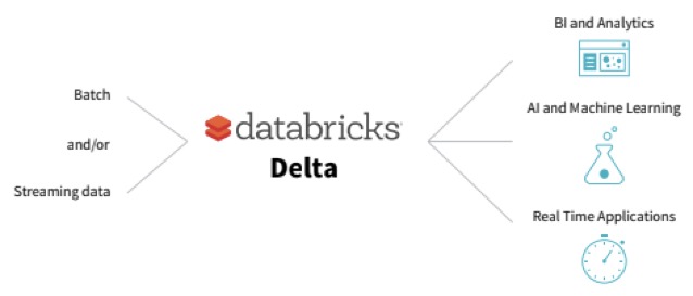
Using an innovative new table design, Delta supports both batch and streaming use cases with high query performance and strong data reliability while requiring a simpler data pipeline architecture:
Increased query performance – Able to deliver 10 to 100 times faster performance than Apache Spark(™) on Parquet through the use of key enablers such as compaction, flexible indexing, multi-dimensional clustering and data caching.
Improved data reliability – By employing ACID (“all or nothing”) transactions, schema validation / enforcement, exactly once semantics, snapshot isolation and support for UPSERTS and DELETES.
Reduced system complexity – Through the unification of batch and streaming in a common pipeline architecture – being able to operate on the same table also means a shorter time from data ingest to query result. Schema evolution provides the ability to infer schema from input data making it easier to deal with changing business needs.
Delta can be deployed to help address a myriad of use cases including IoT, clickstream analytics and cyber security. Indeed, some of our customers are already finding value with Delta for these – I hope to share more on that in future posts. My colleagues have written a blog (Simplify Streaming Stock Data Analysis Using Databricks Delta) to showcase Delta that you might interesting.
Porting existing Spark code for using Delta is as simple as changing
“CREATE TABLE … USING parquet” to
“CREATE TABLE … USING delta”
or changing
“dataframe.write.format(“parquet“).load(“/data/events“)”
“dataframe.write.format(“delta“).load(“/data/events“)”
If you are already using Azure Databricks Premium you can explore Delta today using:
If you are not already using Databricks, you can try Databricks Delta for free by signing up for the free Azure Databricks 14 day trial.
You can learn more about Delta from the Databricks Delta documentation.
--
Try Databricks for free. Get started today.
The post Databricks Delta: Now Available in Preview as Part of Microsoft Azure Databricks appeared first on Databricks.

If you’ve any interest in writing nicely then a $1 ballpoint won’t cut it, you need to look at a fountain pen.
Unlike a lot of our guid…

Roku just added a couple of killer little pieces to its already strong catalog of streaming devices with the new $40 Premiere and $50 Premiere+…

T-Mobile’s prepaid brand MetroPCS is getting a new name: Metro by T-Mobile.

Two out of two Review Geek staffers agree: the second “e” in “rechargeable” is awkward and unnecessary.

If you’re looking for a cross between the easy comfort of a bean bag chair and the support of desk chair, gaming “rocker” ch…
In part 2 of our series on MLflow blogs, we demonstrated how to use MLflow to track experiment results for a Keras network model using binary classification. We classified reviews from an IMDB dataset as positive or negative. And we created one baseline model and two experiments. For each model, we tracked its respective training accuracy and loss and validation accuracy and loss.
In this third part in our series, we’ll show how you can save your model, reproduce results, load a saved model, predict unseen reviews—all easily with MLFlow—and view results in TensorBoard.
MLflow logging APIs allow you to save models in two ways. First, you can save a model on a local file system or on a cloud storage such as S3 or Azure Blob Storage; second, you can log a model along with its parameters and metrics. Both preserve the Keras HDF5 format, as noted in MLflow Keras documentation.
First, if you save the model using MLflow Keras model API to a store or filesystem, other ML developers not using MLflow can access your saved models using the generic Keras Model APIs. For example, within your MLflow runs, you can save a Keras model as shown in this sample snippet:
import mlflow.keras
#your Keras built, trained, and tested model
model = ...
#local or remote S3 or Azure Blob path
model_dir_path=...
# save the mode to local or remote accessible path on the S3 or Azure Blob
mlflow.keras.save_model(model, model_dir_path)
Once saved, ML developers outside MLflow can simply use the Keras APIs to load the model and predict it. For example,
import keras
from keras.models import load_model

model_dir_path = ...
new_data = ...
model = load_model(model_dir_path)
predictions = model.predict(new_data)
Second, you can save the model as part of your run experiments, along with other metrics and artifacts as shown in the code snippet below:
import mlflow
import mlfow.keras
#your Keras built, trained, and tested model
model = ...
with mlflow.start_run():
   # log metrics
   mlflow.log_metric("binary_loss", binary_loss)
   mlflow.log_metric("binary_acc", binary_acc)
   mlflow.log_metric("validation_loss", validation_loss)
   mlflow.log_metric("validation_acc", validation_acc)
   mlflow.log_metric("average_loss", average_loss)
   mlflow.log_metric("average_acc", average_acc)
   # log artifacts
   mlflow.log_artifacts(image_dir, "images")
   # log model
   mlflow.keras.log_model(model, "models")
With this second approach, you can access its run_uuid or location from the MLflow UI runs as part of its saved artifacts:
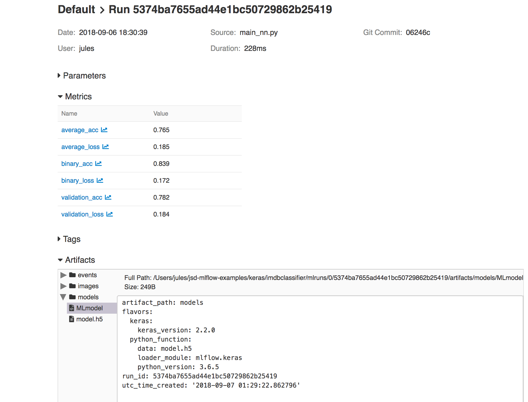
Fig 1. MLflow UI showing artifacts and Keras model saved
In our IMDB example, you can view code for both modes of saving in train_nn.py, class KTrain(). Saving model in this way provides access to reproduce the results from within MLflow platform or reload the model for further predictions, as we’ll show in the sections below.
As part of machine development life cycle, reproducibility of any model experiment by ML team members is imperative. Often you will want to either retrain or reproduce a run from several past experiments to review respective results for sanity, audibility or curiosity.
One way, in our example, is to manually copy logged hyper-parameters from the MLflow UI for a particular run_uuid and rerun using main_nn.py or reload_nn.py with the original parameters as arguments, as explained in the README.md.
Either way, you can reproduce your old runs and experiments:
python reproduce_run_nn.py --run_uuid=5374ba7655ad44e1bc50729862b25419
python reproduce_run_nn.py --run_uuid=5374ba7655ad44e1bc50729862b25419 [--tracking_server=URI]
Or use mlflow run command:
mlflow run keras/imdbclassifier -e reproduce -P run_uuid=5374ba7655ad44e1bc50729862b25419
mlflow run keras/imdbclassifier -e reproduce -P run_uuid=5374ba7655ad44e1bc50729862b25419 [-P tracking_server=URI]
By default, the tracking_server defaults to the local mlruns directory. Here is an animated sample output from a reproducible run:
Fig 2. Run showing reproducibility from a previous run_uuid: 5374ba7655ad44e1bc50729862b25419
In the previous sections, when executing your test runs, the models used for these test runs also saved via the mlflow.keras.log_model(model, "models"). Your Keras model is saved in HDF5 file format as noted in MLflow > Models > Keras. Once you have found a model that you like, you can re-use your model using MLflow as well.
This model can be loaded back as a Python Function as noted noted in mlflow.keras using mlflow.keras.load_model(path, run_id=None).
To execute this, you can load the model you had saved within MLflow by going to the MLflow UI, selecting your run, and copying the path of the stored model as noted in the screenshot below.
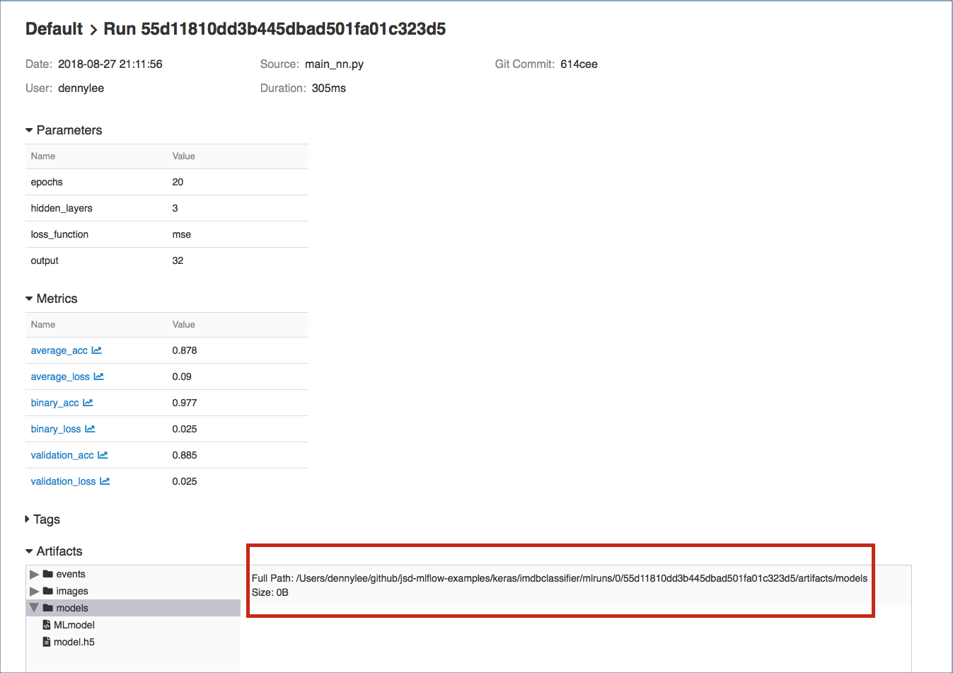
Fig 3. MLflow model saved in the Artifacts
With your model identified, you can type in your own review by loading your model and executing it. For example, let’s use a review that is not included in the IMDB Classifier dataset:
this is a wonderful film with a great acting, beautiful cinematography, and amazing direction
To run a prediction against this review, use the predict_nn.py against your model:
python predict_nn.py --load_model_path='/Users/dennylee/github/jsd-mlflow-examples/keras/imdbclassifier/mlruns/0/55d11810dd3b445dbad501fa01c323d5/artifacts/models' --my_review='this is a wonderful film with a great acting, beautiful cinematography, and amazing direction'
Or you can run it directly using mlflow and the imdbclassifer repo package:
mlflow run keras/imdbclassifier -e predict -P load_model_path='/Users/jules/jsd-mlflow-examples/keras/imdbclassifier/keras_models/178f1d25c4614b34a50fbf025ad6f18a' -P my_review='this is a wonderful film with a great acting, beautiful cinematography, and amazing direction'
The output for this command should be similar to the following output predicting a positive sentiment for the provided review.
Using TensorFlow backend.
load model path: /tmp/models
my review: this is a wonderful film with a great acting, beautiful cinematography, and amazing direction
verbose: False
Loading Model...
Predictions Results:
[[ 0.69213998]]
In addition to reviewing your results in the MLflow UI, the code samples save TensorFlow events so that you can visualize the TensorFlow session graph. For example, after executing the statement python main_nn.py, you will see something similar to the following output:
Average Probability Results:
[0.30386349968910215, 0.88336000000000003]

Predictions Results:
[[ 0.35428655]
[ 0.99231517]
[ 0.86375767]
...,
[ 0.15689197]
[ 0.24901576]
[ 0.4418138 ]]
Writing TensorFlow events locally to /var/folders/0q/c_zjyddd4hn5j9jkv0jsjvl00000gp/T/tmp7af2qzw4

Uploading TensorFlow events as a run artifact.
loss function use binary_crossentropy
This model took 51.23427104949951 seconds to train and test.
You can extract the TensorBoard log directory with the output line stating Writing TensorFlow events locally to .... And to start TensorBoard, you can run the following command:
tensorboard --logdir=/var/folders/0q/c_zjyddd4hn5j9jkv0jsjvl00000gp/T/tmp7af2qzw4
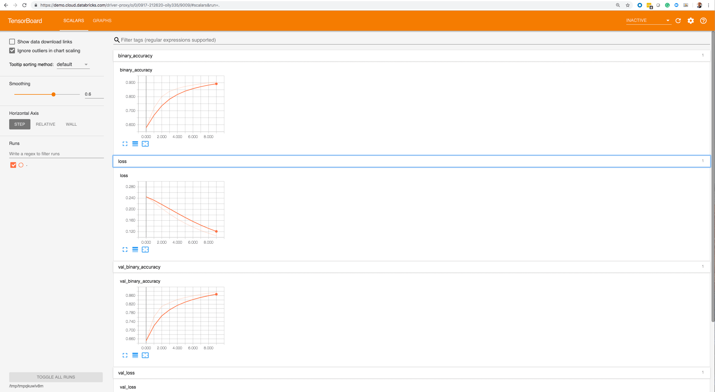

Within the TensorBoard UI:
In this blog post, we demonstrated how to use MLflow to save models and reproduce results from saved models as part of the machine development life cycle. In addition, through both python and mlflow command line, we loaded a saved model and predicted the sentiment of our own custom review unseen by the model. Finally, we showcased how you can utilize MLflow and TensorBoard side-by-side by providing code samples that generate TensorFlow events so you can visualize the metrics as well as the session graph.
You have seen, in three parts, various aspects of MLflow: from experimentation to reproducibility and using MLlfow UI and TensorBoard for visualization of your runs.
You can try MLflow at mlflow.org to get started. Or try some of tutorials and examples in the documentation, including our example notebook Keras_IMDB.py for this blog.
Here are some resources for you to learn more:
--
Try Databricks for free. Get started today.
The post How to Use MLflow To Reproduce Results and Retrain Saved Keras ML Models appeared first on Databricks.

Whether you’ve just moved out on your own for the first time or you’re finally getting serious about cooking, we’ve rounded…

Ultrawide monitors are designed to give you ample room in your workspace without having to set up two separate monitors.

Amazon dropped a positively massive new batch of Alexa-enabled and smart home devices, from subwoofers to microwaves.
If data is the new bacon, data stewardship supplies its nutrition label! This is the second part of a two-part blog introducing Data Steward Studio (DSS) which covers a detailed walkthrough of the capabilities in Data Steward Studio With GDPR coming into effect in May 2018 and California legislature signing California Consumer Privacy Act […]
The post DISCOVER with Data Steward Studio (DSS): Understand your your hybrid data lakes to exploit their business value! Part-2 appeared first on Hortonworks.

Starting next year, the PS Vita will be discontinued in Japan, officially ending its lifespan. What comes next? According to Sony, nothing.

The PS4 is currently king of the consoles, boasting enviable exclusives like Spider-Man, God of War, and Horizon: Zero D…
Introduction The Apache Hadoop community announced Hadoop 3.0 GA in December, 2017 and Hadoop 3.1 in April, 2018 loaded with great features and improvements. One of the biggest challenges while upgrading to a new major release of a software platform is its compatibility. Apache Hadoop community has focused on ensuring wire and binary compatibility for […]
The post Upgrading your clusters and workloads from Hadoop 2 to Hadoop 3 appeared first on Hortonworks.
The Nintendo Switch Online service is live and we finally got to try it out.

Most Bluetooth headphones sold today include a microphone in their housing, allowing them to make and answer calls.
We’ve just published our most recent customer video! This video gives a look at how Micron is able to focus more on building solutions and less on day-to-day data management through partnering with Hortonworks. Micron Technology, Inc. is an American global corporation based in Boise, Idaho. The company is one of the largest memory manufacturers in the […]
The post How Micron is Achieving Faster Insights, Developing Analytical Solutions appeared first on Hortonworks.

If you want to drink more water, get more out of your health apps, and feel better in the proc…
How is Apache Metron utilized in Hortonworks’ product portfolio? Hortonworks Cybersecurity Platform (HCP) is powered by Apache Metron and other open-source big data technologies. At the prime intersection of Big Data and Machine Learning, HCP employs a data-science-based approach to visualize diverse, streaming security data at scale to aid Security Operations Centers (SOC) in real-time detection […]
The post Q&A to Demystify the Power of Apache Metron in Real-Time Threat Detection appeared first on Hortonworks.
When I first wrote about Jenkins Evergreen, which was then referred to as "Jenkins Essentials", I mentioned a number of future developments which in the subsequent months have become reality. At this year’s DevOps World - Jenkins World in San Francisco, I will be sharing more details on the philosophy behind Jenkins Evergreen, show off how far we have come, and discuss where we’re going with this radical distribution of Jenkins.

As discussed in my first blog post, and JEP-300, the first two pillars of Jenkins Evergreen have been the primary focus of our efforts.
Perhaps unsurprisingly, implementing the mechanisms necessary for safely and automatically updating a Jenkins distribution, which includes core and plugins, was and continues to be a sizable amount of work. In Baptiste’s talk he will be speaking about the details which make Evergreen "go" whereas I will be speaking about why an automatically updating distribution is important.
As continuous integration and continuous delivery have become more commonplace, and fundamental to modern software engineering, Jenkins tends to live two different lifestyles depending on the organization. In some organizations, Jenkins is managed and deployed methodically with automation tools like Chef, Puppet, etc. In many other organizations however, Jenkins is treated much more like an appliance, not unlike the office wireless router. Installed and so long as it continues to do its job, people won’t think about it too much.
Jenkins Evergreen’s distribution makes the "Jenkins as an Appliance" model much better for everybody by ensuring the latest feature updates, bug and security fixes are always installed in Jenkins.
Additionally, I believe Evergreen will serve another group we don’t adequately serve at the moment: those who want Jenkins to behave much more like a service. We typically don’t consider "versions" of GitHub.com, we receive incremental updates to the site and realize the benefits of GitHub’s on-going development without ever thinking about an "upgrade."
I believe Jenkins Evergreen can, and will provide that same experience.
The really powerful thing about Jenkins as a platform is the broad variety of patterns and practices different organizations may adopt. For newer users, or users with common use-cases, that significant amount of flexibility can result in a paradox of choice. With Jenkins Evergreen, much of the most common configuration is automatically configured out of the box.
Included is Jenkins Pipeline and Blue Ocean, by default. We also removed some legacy functionalities from Jenkins while we were at it.
We are also utilizing some of the fantastic Configuration as Code work, which recently had its 1.0 release, to automatically set sane defaults in Jenkins Evergreen.
The effort has made significant strides thus far this year, and we’re really excited for people to start trying out Jenkins Evergreen. As of today, Jenkins Evergreen is ready for early adopters. We do not yet recommend using Jenkins Evergreen for a production environment.
If you’re at DevOps World - Jenkins World in San Francisco please come see Baptiste’s talk Wednesday at 3:45pm in Golden Gate Ballroom A. Or my talk at 11:15am in Golden Gate Ballroom B.
If you can’t join us here in San Francisco, we hope to hear your feedback and thoughts in our Gitter channel!

There’s a lot of factors to consider when selecting a voice-assistant platform but what if your biggest consideration is just how they a…

Street photography is one of the most popular forms of photography for people to start with.
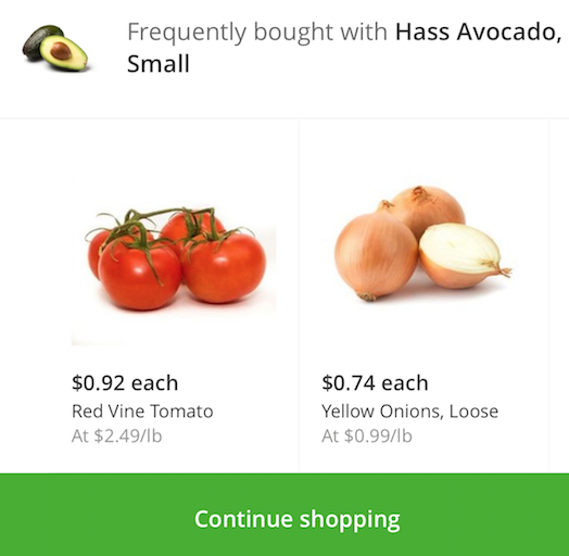
When providing recommendations to shoppers on what to purchase, you are often looking for items that are frequently purchased together (e.g. peanut butter and jelly). A key technique to uncover associations between different items is known as market basket analysis. In your recommendation engine toolbox, the association rules generated by market basket analysis (e.g. if one purchases peanut butter, then they are likely to purchase jelly) is an important and useful technique. With the rapid growth e-commerce data, it is necessary to execute models like market basket analysis on increasing larger sizes of data. That is, it will be important to have the algorithms and infrastructure necessary to generate your association rules on a distributed platform. In this blog post, we will discuss how you can quickly run your market basket analysis using Apache Spark MLlib FP-growth algorithm on Databricks.
To showcase this, we will use the publicly available Instacart Online Grocery Shopping Dataset 2017. In the process, we will explore the dataset as well as perform our market basket analysis to recommend shoppers to buy it again or recommend to buy new items.

The flow of this post, as well as the associated notebook, is as follows: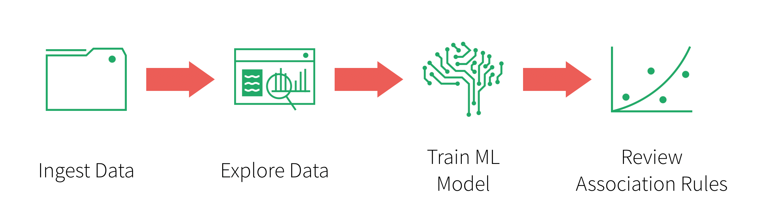
The dataset we will be working with is 3 Million Instacart Orders, Open Sourced dataset:
The “Instacart Online Grocery Shopping Dataset 2017”, Accessed from https://www.instacart.com/datasets/grocery-shopping-2017 on 01/17/2018. This anonymized dataset contains a sample of over 3 million grocery orders from more than 200,000 Instacart users. For each user, we provide between 4 and 100 of their orders, with the sequence of products purchased in each order. We also provide the week and hour of day the order was placed, and a relative measure of time between orders.
You will need to download the file, extract the files from the gzipped TAR archive, and upload them into Databricks DBFS using the Import Data utilities. You should see the following files within dbfs once the files are uploaded:
Orders: 3.4M rows, 206K usersProducts: 50K rowsAisles: 134 rowsDepartments: 21 rowsorder_products__SET: 30M+ rows where SET is defined as:
prior: 3.2M previous orderstrain: 131K orders for your training datasetRefer to the Instacart Online Grocery Shopping Dataset 2017 Data Descriptions for more information including the schema.
Now that you have uploaded your data to dbfs, you can quickly and easily create your DataFrames using spark.read.csv:
# Import Data
aisles = spark.read.csv("/mnt/bhavin/mba/instacart/csv/aisles.csv", header=True, inferSchema=True)
departments = spark.read.csv("/mnt/bhavin/mba/instacart/csv/departments.csv", header=True, inferSchema=True)
order_products_prior = spark.read.csv("/mnt/bhavin/mba/instacart/csv/order_products__prior.csv", header=True, inferSchema=True)
order_products_train = spark.read.csv("/mnt/bhavin/mba/instacart/csv/order_products__train.csv", header=True, inferSchema=True)
orders = spark.read.csv("/mnt/bhavin/mba/instacart/csv/orders.csv", header=True, inferSchema=True)
products = spark.read.csv("/mnt/bhavin/mba/instacart/csv/products.csv", header=True, inferSchema=True)

# Create Temporary Tables
aisles.createOrReplaceTempView("aisles")
departments.createOrReplaceTempView("departments")
order_products_prior.createOrReplaceTempView("order_products_prior")
order_products_train.createOrReplaceTempView("order_products_train")
orders.createOrReplaceTempView("orders")
products.createOrReplaceTempView("products")
Now that you have created DataFrames, you can perform exploratory data analysis using Spark SQL. The following queries showcase some of the quick insight you can gain from the Instacart dataset.
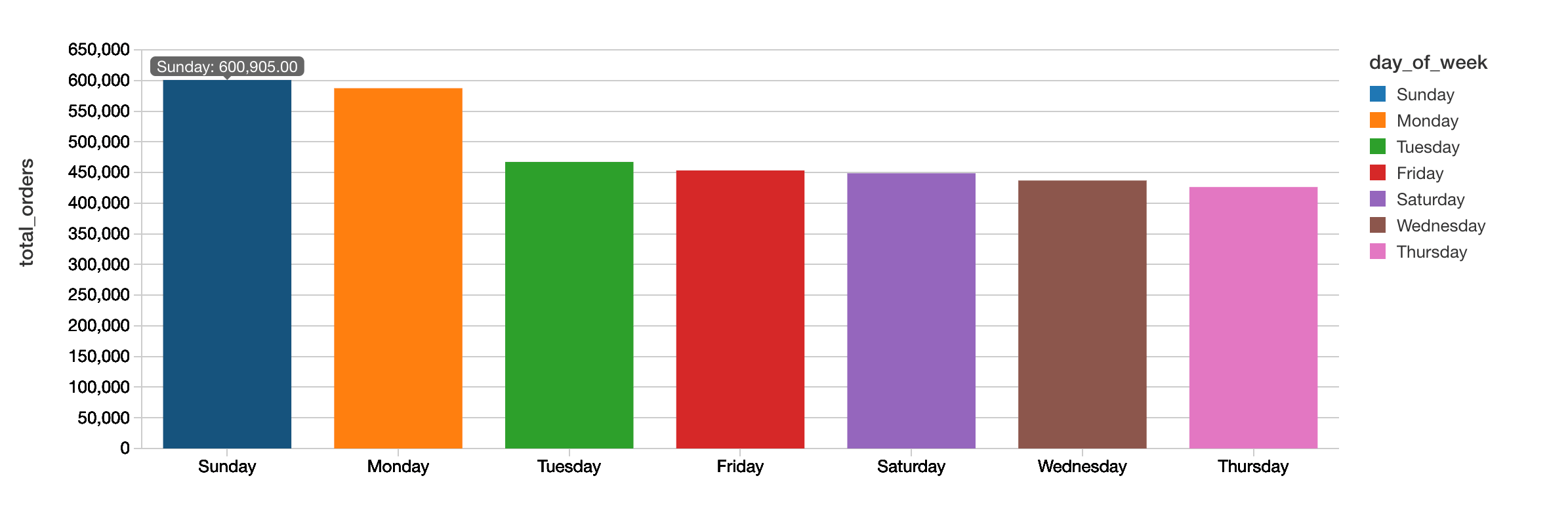
The following query allows you to quickly visualize that Sunday is the most popular day for the total number of orders while Thursday has the least number of orders.
%sql
select
  count(order_id) as total_orders,
  (case
     when order_dow = '0' then 'Sunday'
     when order_dow = '1' then 'Monday'
     when order_dow = '2' then 'Tuesday'
     when order_dow = '3' then 'Wednesday'
     when order_dow = '4' then 'Thursday'
     when order_dow = '5' then 'Friday'
     when order_dow = '6' then 'Saturday'
   end) as day_of_week
  from orders
 group by order_dow
 order by total_orders desc
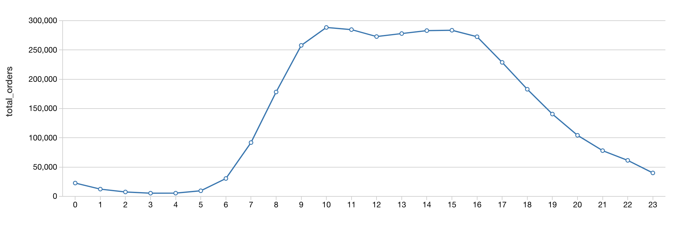
When breaking down the hours typically people are ordering their groceries from Instacart during business working hours with highest number orders at 10:00am.
%sql
select
  count(order_id) as total_orders,
  order_hour_of_day as hour
  from orders
 group by order_hour_of_day
 order by order_hour_of_day
As we dive deeper into our market basket analysis, we can gain insight on the number of products by department to understand how much shelf space is being used.
%sql
select d.department, count(distinct p.product_id) as products
  from products p
    inner join departments d
      on d.department_id = p.department_id
 group by d.department
 order by products desc
 limit 10
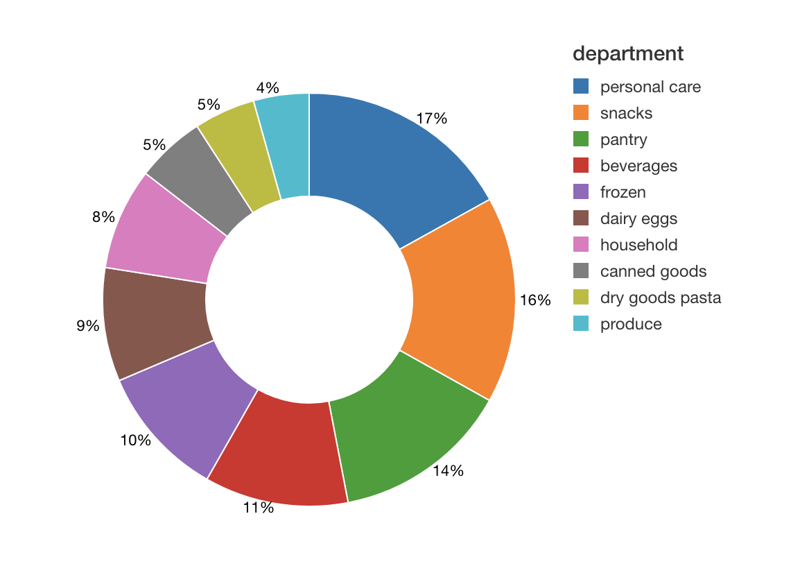
As can see from the preceding image, typically the number of unique items (i.e. products) involve personal care and snacks.
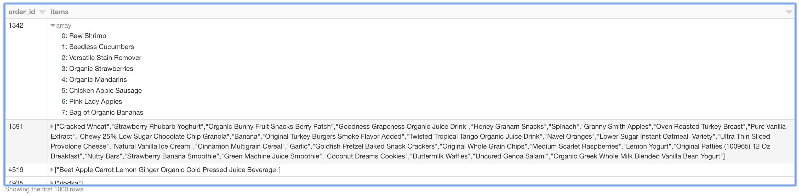
To prepare our data for downstream processing, we will organize our data by shopping basket. That is, each row of our DataFrame represents an order_id with each items column containing an array of items.
# Organize the data by shopping basket
from pyspark.sql.functions import collect_set, col, count
rawData = spark.sql("select p.product_name, o.order_id from products p inner join order_products_train o where o.product_id = p.product_id")
baskets = rawData.groupBy('order_id').agg(collect_set('product_name').alias('items'))
baskets.createOrReplaceTempView('baskets')
Just like the preceding graphs, we can visualize the nested items using thedisplay command in our Databricks notebooks.
To understand the frequency of items are associated with each other (e.g. how many times does peanut butter and jelly get purchased together), we will use association rule mining for market basket analysis. Spark MLlib implements two algorithms related to frequency pattern mining (FPM): FP-growth and PrefixSpan. The distinction is that FP-growth does not use order information in the itemsets, if any, while PrefixSpan is designed for sequential pattern mining where the itemsets are ordered. We will use FP-growth as the order information is not important for this use case.
Note, we will be using the
Scala APIso we can configuresetMinConfidence
%scala
import org.apache.spark.ml.fpm.FPGrowth

// Extract out the items
val baskets_ds = spark.sql("select items from baskets").as[Array[String]].toDF("items")

// Use FPGrowth
val fpgrowth = new FPGrowth().setItemsCol("items").setMinSupport(0.001).setMinConfidence(0)
val model = fpgrowth.fit(baskets_ds)

// Calculate frequent itemsets
val mostPopularItemInABasket = model.freqItemsets
mostPopularItemInABasket.createOrReplaceTempView("mostPopularItemInABasket")
With Databricks notebooks, you can use the
%scalato execute Scala code within a new cell in the same Python notebook.
With the mostPopularItemInABasket DataFrame created, we can use Spark SQL to query for the most popular items in a basket where there are more than 2 items with the following query.
%sql
select items, freq from mostPopularItemInABasket where size(items) > 2 order by freq desc limit 20
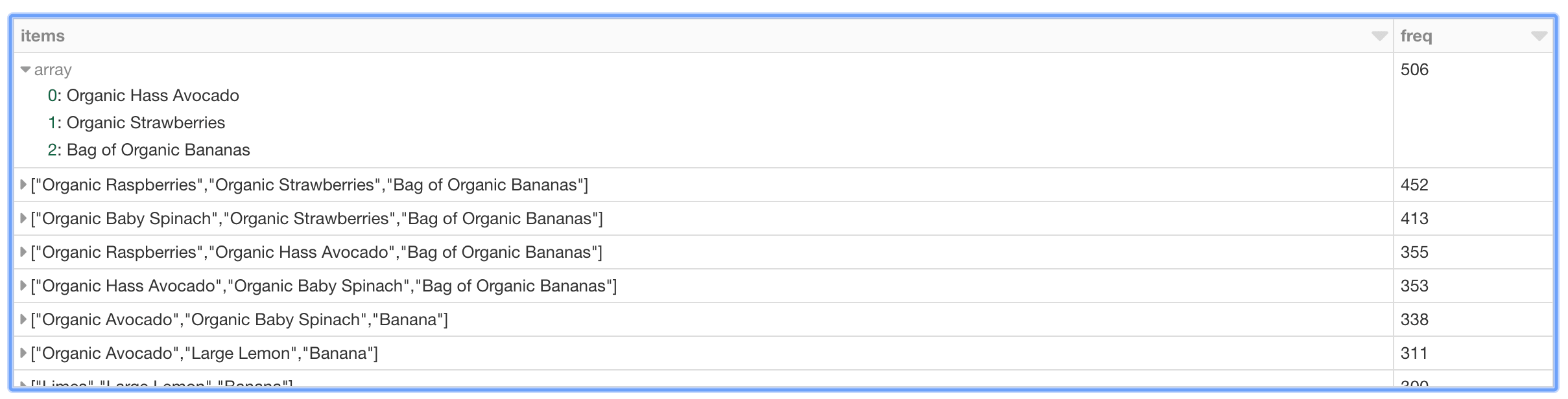
As can be seen in the preceding table, the most frequent purchases of more than two items involve organic avocados, organic strawberries, and organic bananas. Interesting, the top five frequently purchased together items involve various permutations of organic avocados, organic strawberries, organic bananas, organic raspberries, and organic baby spinach. From the perspective of recommendations, the freqItemsets can be the basis for the buy-it-again recommendation in that if a shopper has purchased the items previously, it makes sense to recommend that they purchase it again.
In addition to freqItemSets, the FP-growth model also generates associationRules. For example, if a shopper purchases peanut butter, what is the probability (or confidence) that they will also purchase jelly. For more information, a good reference is Susan Li’s A Gentle Introduction on Market Basket Analysis — Association Rules.
%scala
// Display generated association rules.
val ifThen = model.associationRules
ifThen.createOrReplaceTempView("ifThen")
A good way to think about association rules is that model determines that if you purchased something (i.e. the antecedent), then you will purchase this other thing (i.e. the consequent) with the following confidence.
%sql
select antecedent as `antecedent (if)`, consequent as `consequent (then)`, confidence from ifThen order by confidence desc limit 20
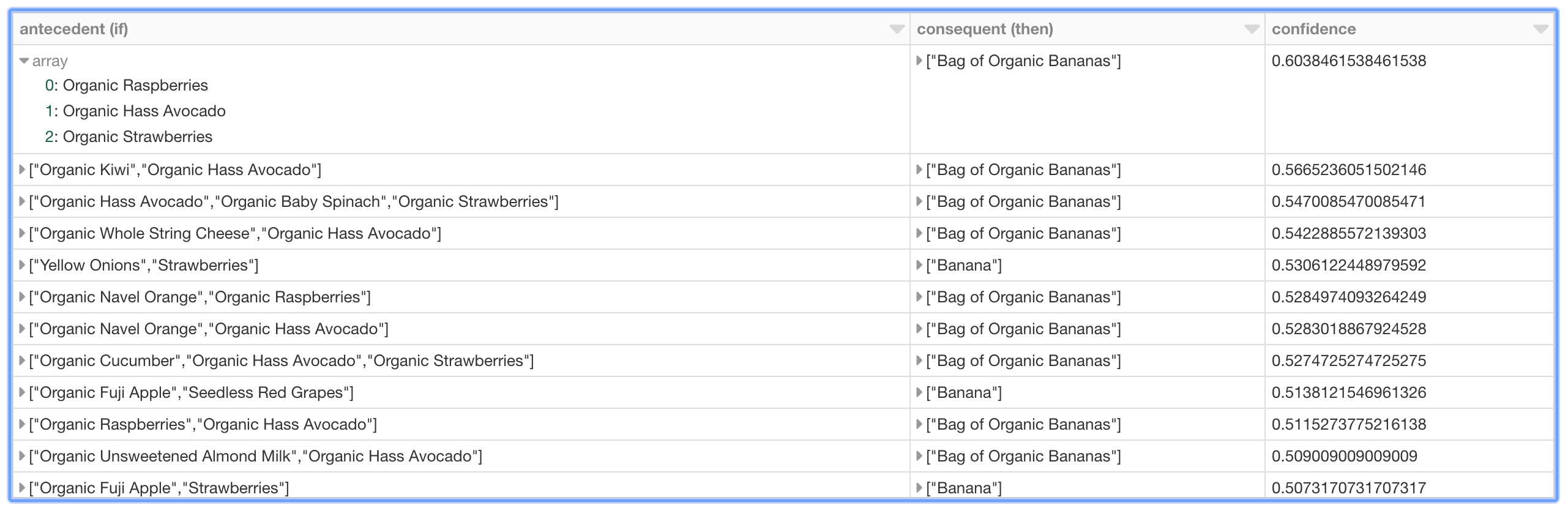
As can be seen in the preceding graph, there is relatively strong confidence that if a shopper has organic raspberries, organic avocados, and organic strawberries in their basket, then it may make sense to recommend organic bananas as well. Interestingly, the top 10 (based on descending confidence) association rules – i.e. purchase recommendations – are associated with organic bananas or bananas.
In summary, we demonstrated how to explore our shopping cart data and execute market basket analysis to identify items frequently purchased together as well as generating association rules. By using Databricks, in the same notebook we can visualize our data; execute Python, Scala, and SQL; and run our FP-growth algorithm on an auto-scaling distributed Spark cluster – all managed by Databricks. Putting these components together simplifies the data flow and management of your infrastructure for you and your data practitioners. Try out the Market Basket Analysis using Instacart Online Grocery Dataset with Databricks today.
--
Try Databricks for free. Get started today.
The post Simplify Market Basket Analysis using FP-growth on Databricks appeared first on Databricks.


